Day 2: Using a Supercomputer

You do not necessarily need to know how a supercomputer is organized in order to use one. Still, if you are going to use a supercomputer, it is worth learning briefly what one is. As often happens with words like this, however, what qualifies as a “supercomputer” varies greatly from person to person. The explanation here is only the author’s definition; others may have different definitions. Rather than teaching you how to accomplish a particular task, this chapter presents things that someone who has never used a supercomputer will probably benefit from knowing before doing so. There are no hands-on exercises. Feel free to read it casually as background material.

What Is a Supercomputer?

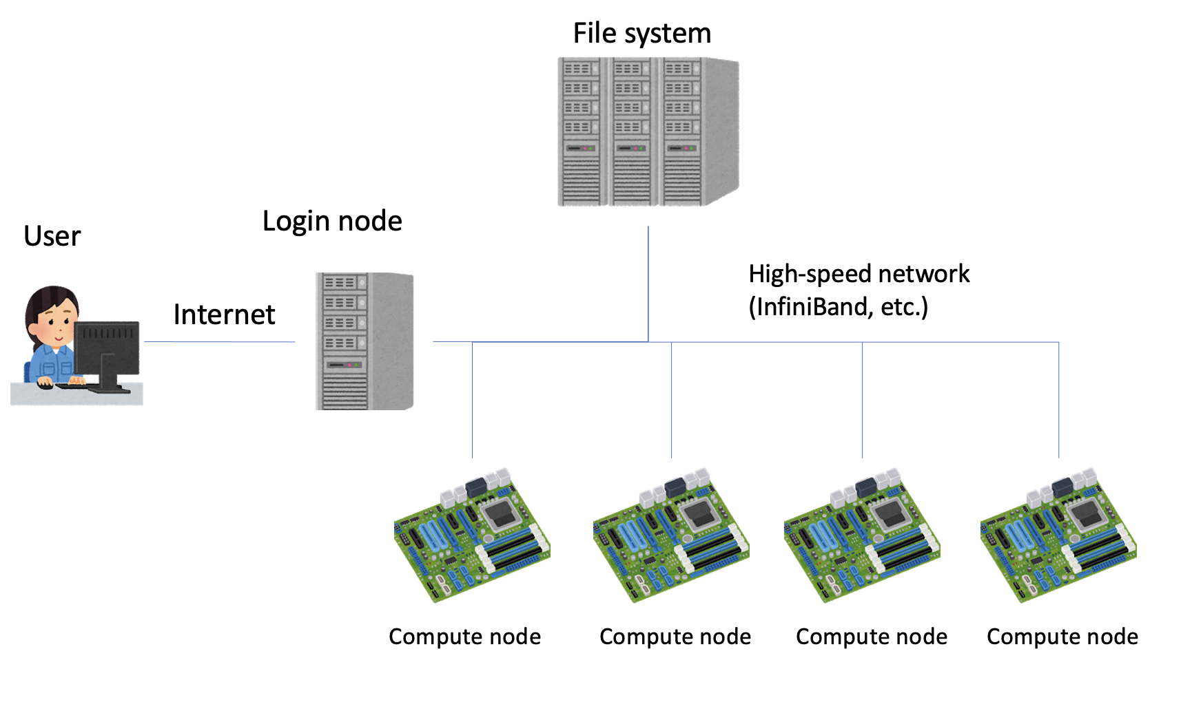
An ordinary PC consists of a CPU, memory, a network interface, disks, and so on. A supercomputer likewise has CPUs, memory, a network, and disks. The individual parts are somewhat higher-end, but fundamentally they are the same as those in an ordinary PC. What differs is how they are connected. In a supercomputer, a CPU and its memory together are called a node. The main body of the supercomputer consists of many such nodes connected by a high-speed network. An ordinary PC has storage near its CPU, but modern supercomputer nodes are often diskless and instead connect over the network to a large file system.

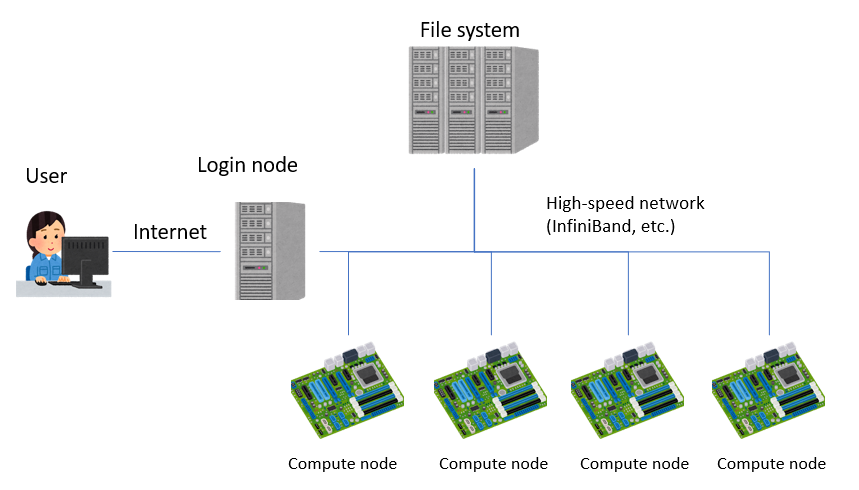
The diagram above shows a typical supercomputer. Nodes fall broadly into two types: login nodes and compute nodes. Users log in to a login node over the Internet and work there, while actual calculations run on compute nodes. Login nodes, compute nodes, and the file system are joined by a high-speed network. InfiniBand was long the de facto standard for this network, although Intel Omni-Path has also seen increasing adoption in recent years. Lustre is the de facto standard file system, while alternatives such as GPFS—now apparently renamed IBM Spectrum Scale—may be chosen for some purposes.

Although we call them nodes, they are essentially computers. A supercomputer can thus be described as a great many computers connected to one another by a high-speed network. The recent prevalence of x86 CPUs reinforces the impression that it is simply a large collection of ordinary PCs. Nevertheless, putting many ordinary PCs side by side does not by itself make a supercomputer. The single most important property of a supercomputer is reliability.

Anyone who uses PCs regularly knows that their components fail fairly often. Any part can fail, but moving parts such as fans and disks are especially vulnerable. Memory is another common source of failures; CPUs, motherboards, and network cards fail too. Because a supercomputer contains so many components, even a very rare failure at the component level becomes non-negligible for the system as a whole.

For example, when the K computer achieved 10 petaflops, the calculation used 88,128 nodes and took 29 hours and 28 minutes. That is approximately 2.6 million node-hours. For the calculation to complete successfully with 90% probability, each node would need to be “guaranteed” not to fail for roughly 3,000 years. Conversely, if each node failed about once per year, some node would fail roughly once every six minutes and the machine would be unusable.

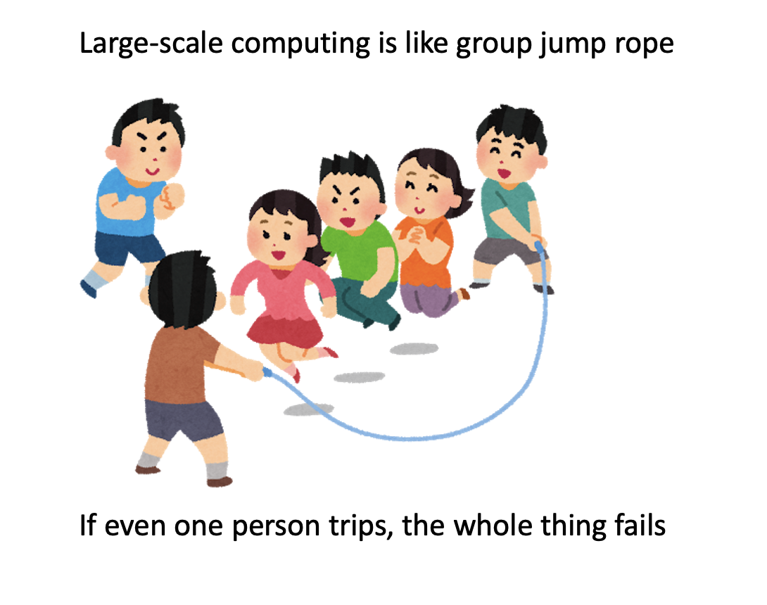
Large-scale computing is therefore like a team jump-rope exercise: doing useful calculations with a substantial number of nodes requires an extremely reliable system. Supercomputers have many other distinctive qualities and engineering techniques, but high reliability is crucial above all. News occasionally appears about a “budget supercomputer” built from game consoles or inexpensive chips. In reality, a substantial portion of a supercomputer’s cost lies not only in its compute units but also in reliability and networking. Cutting costs there naturally produces a machine unable to perform calculations that require those properties. If your desired calculation works on a budget supercomputer, then by all means choose one. But do not compare only peak performance and price and immediately conclude that supercomputers are expensive. As The Little Prince says, what is essential is invisible to the eye.

Aside: Memory Errors on Blue Gene/L

We have seen that failures become a problem because a supercomputer has so many components. Other phenomena that rarely matter on an ordinary PC can also become significant on a supercomputer. One is cosmic radiation.

Cosmic rays are literally radiation arriving from outer space. If you visit a science museum, take a look at a cloud-chamber exhibit. Although we are normally unaware of them, cosmic rays are constantly flying through us. When they strike semiconductor devices, they can cause malfunctions. Memory is particularly vulnerable: a cosmic ray can randomly flip a bit and corrupt a result. To prevent this, memory commonly provides error correction that can correct a one-bit error and detect a two-bit error.

One supercomputer lacked this capability: IBM’s Blue Gene/L. Blue Gene’s design sought to combine high overall performance with low power consumption by connecting a large number of relatively modest nodes. Bold simplifications appeared throughout the system—for example, the compute-node OS did not support multiple users. Most surprising was the absence of error correction in the CPU’s L1 cache. Blue Gene/L’s L1 cache could detect a one-bit error but could not correct it. A bit error therefore caused the system to crash.

According to a manual from Lawrence Livermore National Laboratory, which installed Blue Gene/L, a full-machine calculation on 200,000 cores was estimated to crash from a cosmic-ray-induced L1 bit error about once every six hours on average. Users had three options:

• Give up: six hours applies to the full machine, so a calculation using, for example, 10,000 cores would have a mean time between failures of about 120 hours. Simply running the calculation and accepting an occasional failure was a realistic choice.
• Use memory-protection mode: Blue Gene/L offered a “write-through mode” that apparently protected against L1 bit errors in software by using L2 cache or main memory. It required no user intervention, but reportedly reduced performance by about 10% to 40%.
• Receive an exception and handle it in the application: in this mode, the OS raised an exception when L1 detected a bit error, leaving recovery to the user.

Users normally either accepted the risk or used write-through mode when its performance penalty was tolerable. The Livermore team that ran a long full-machine Blue Gene/L calculation and won the 2007 Gordon Bell Prize chose to handle exceptions in its own application. Specifically, they kept checkpoint data in part of memory and wrote code that restarted from the latest checkpoint after receiving an exception. According to their paper, the approximately three-day full-machine calculation received exceptions and restarted several times. I once spoke with a member of the team and remember hearing that making recovery safe regardless of where in the program an exception arrived was difficult.

People have long argued that, as systems grow, hardware alone cannot guarantee reliability and software must handle part of the task. Much research has explored the idea, and some mechanisms have been incorporated experimentally into systems. To the best of my knowledge, however, Blue Gene/L is the only example in which this philosophy was placed into actual production use.

I do not know why L1 error correction was omitted or could not be implemented. Its inclusion in the successor Blue Gene/P suggests that users may not have liked the omission. The Blue Gene series sold quite well in HPC: four of the top ten systems in the June 2007 TOP500 list were Blue Gene machines. Development proceeded from the first-generation Blue Gene/L through the second-generation Blue Gene/P and third-generation Blue Gene/Q, after which the Blue Gene project ended.

Obtaining a Supercomputer Account

To use a supercomputer, you must first obtain an account. In a sense, this is the hardest part. Learning the technology for using a supercomputer is straightforward, but obtaining an account is not a technical skill.

Many kinds of supercomputers exist. Companies install them for development, and cloud providers now offer computing resources that could reasonably be called supercomputers. Hiroshi Yamamoto, the developer of the shogi program Ponanza, lacked sufficient computing resources for machine learning and reportedly asked Sakura Internet to lend him a large amount of compute capacity. Those without that degree of nerve should obtain an account through ordinary procedures.

First, there are university computing centers, traditionally the obvious place to find a supercomputer. Facilities such as the Information Technology Center at the University of Tokyo rent computing resources at quite reasonable rates after an application. They also issue various calls for proposals through which resources may apparently be used free of charge as part of joint research.

The Institute for Solid State Physics limits projects to materials science, but accepted proposals can use its resources free of charge. Be aware that users must generally be master’s students or above—undergraduates are normally ineligible—and applicants must be salaried researchers, meaning postdocs or above.

The K computer, famous from the question “Why can’t it be number two?”, also accepted proposals from the public. Research projects could use it free of charge provided that their results were published. Up to 80,000 nodes and 640,000 cores were waiting for you in Kobe—until operations ended and the system shut down on August 30, 2019. Preparations for its successor were already under way, however, and another major computing resource would begin operating if all went according to plan.

For research use, it is common for users to be master’s students or above and for applicants to be researchers. But some high-school students may want to use a supercomputer too. For such promising young people, Osaka University and Tokyo Tech have held SuperCon, an event resembling a national high-school supercomputing championship. It is a kind of programming contest distinguished by problems large enough to require parallel computing.

In 2014, a high-school student successfully used a supercomputer to find all solutions to the 5×5 magic square. This used the University of Tsukuba’s interdisciplinary cooperative-use program; a first-year high-school student conducted joint research with a professor and made extensive use of the supercomputer.

Tokyo Tech also sought to broaden supercomputer use through its support program for young and female TSUBAME users and still younger users, apparently accepting proposals from university, high-school, and technical-college students.

Frankly, despite Japan’s status as a supercomputing power, it is not easy for a young person to casually decide, “Let’s use a supercomputer.” The door is narrow, but it is open even to high-school students. Without parallel-programming skills, however, people are unlikely to consider using one at all. It seems sensible to quickly learn parallel programming—it is easy anyway—and be ready to use a supercomputer when an opportunity arises.

How Jobs Are Executed

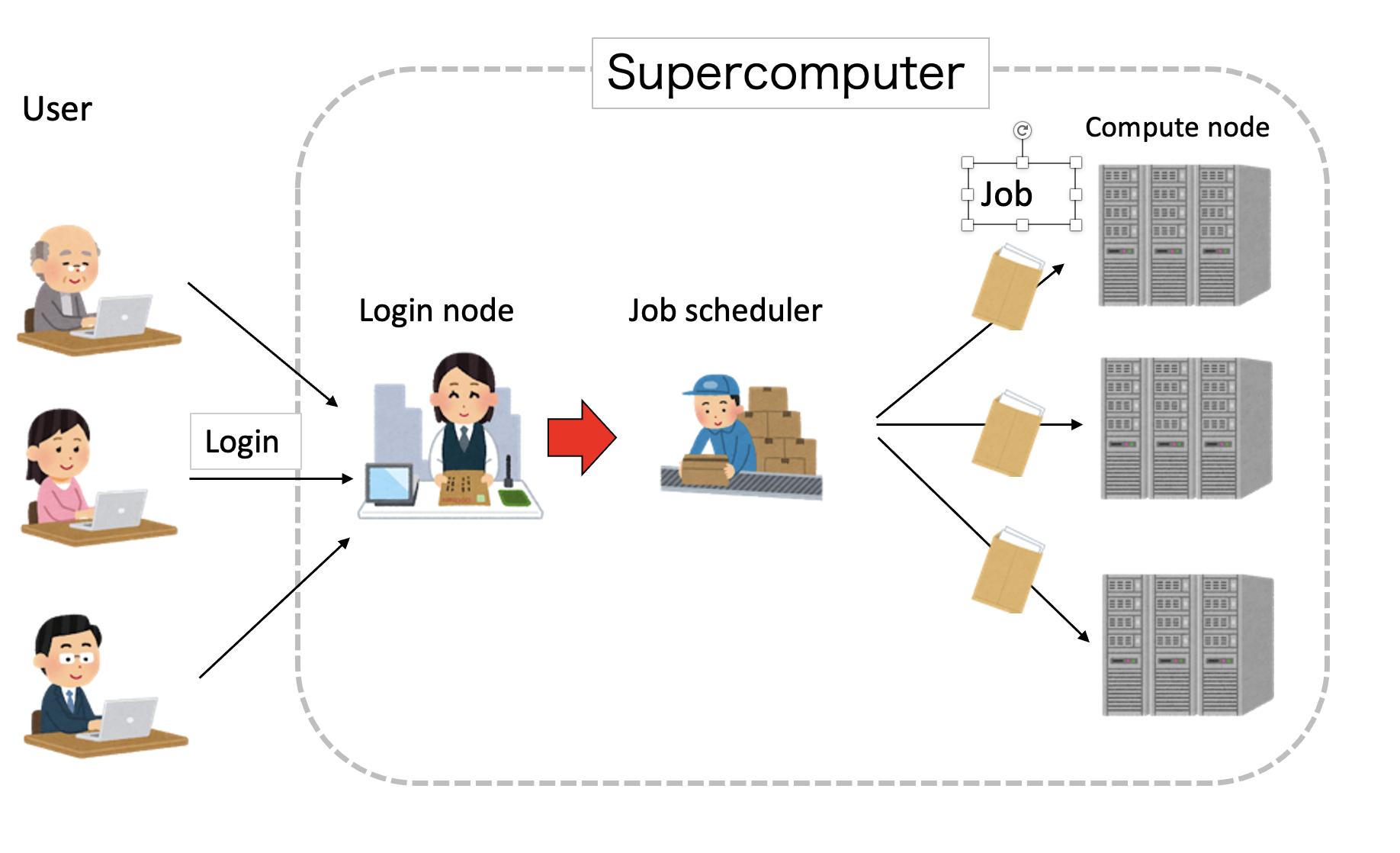
You are the only user of your local PC, so you may run any program whenever you like. A supercomputer, however, is a computing resource shared by many people. Allowing everyone to run programs however they pleased would be disastrous, so some traffic control is necessary. The job scheduler provides that control. Programs on a supercomputer are executed in units called jobs. A user first prepares a shell script called a job script. It is like a letter describing how to run the program. The user then asks the job scheduler from a login node to execute the job, rather like putting an envelope in a mailbox. The job enters a waiting queue. Considering past usage, the requested number of nodes, execution time, and other factors, the scheduler decides which waiting job should run next and where.

Writing a Job Script

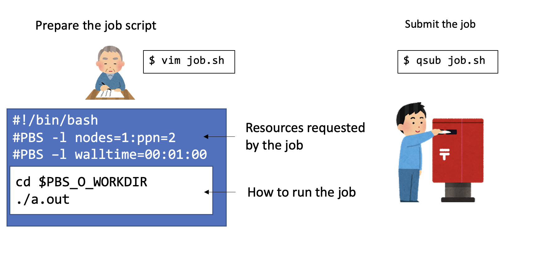
As noted above, programs are compiled and executed in different places on a supercomputer. In addition to an executable, the user prepares a job script and submits it to the scheduler to request execution. The script states the resources the job requires and how it should run. Based on those resources, the scheduler decides when and where to execute it. When its turn arrives, the job script is executed as a shell script and runs the job. The transition of a queued job into the running state is called dispatch.

At the beginning of a job script, resource requests are written as special comments. The precise syntax depends on both the scheduler and the operating policy of the supercomputer site, so consult the site’s documentation when using a real machine. Fundamentally, however, you specify such things as the number of requested nodes and the execution time.

With PBS, one job scheduler, directives follow #PBS. To request two nodes for twelve hours, write:

#PBS -l nodes=2
#PBS -l walltime=12:00:00

Next, describe how to run the job. Remember that it executes on a different machine from the one where you compiled and submitted it. The current directory and environment variables are therefore not inherited. The changed current directory is especially important. You could use an absolute path:

cd /home/path/to/dir
./a.out

Normally, however, the working directory at submission time is stored in a special environment variable. PBS places it in PBS_O_WORKDIR, so you can write:

cd $PBS_O_WORKDIR
./a.out

Specify any other environment variables required for execution as well. Save the resulting script under a name such as go.sh, then pass it to the submission command:

qsub go.sh

The job is now submitted. Use the job-status command—qstat for PBS—to confirm that it is waiting to run.

Some supercomputers contain several kinds of nodes, such as high-memory “fat” nodes or nodes equipped with GPGPUs. In that case, execution units called queues are configured for the different node types, and you should select the appropriate queue.

Fair Share

The scheduler determines the planned time and place of a waiting job. When a preceding job finishes, the job at the head of the queue basically runs next, but many other factors also apply. One important concept is fair share.

Consider a cluster with four compute nodes. User A first submits ten one-node jobs. Four jobs begin running on the four nodes and six enter the queue. User B then submits one one-node job. With simple FIFO scheduling, B’s job goes to the end of the queue. But A already occupies all four nodes, so it seems fair that B’s job should run next. For that to happen, B’s job must overtake jobs that were already queued.

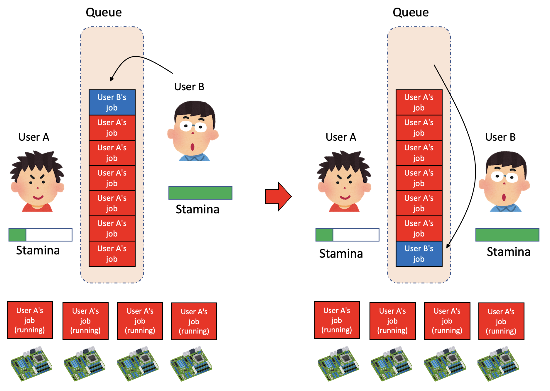
Fair share implements this kind of scheduling. First, assign each user a priority. The more jobs a user runs, the lower their priority becomes; if they have not run a job for some time, it rises again. You can think of it as the stamina meter in a social game. When resources become available, the scheduler selects the highest-priority job capable of using those resources. Users running many jobs therefore lose priority, and a later job submitted by someone who has run few jobs is scheduled first.

What about the instant A’s four jobs start? Almost no computation has yet occurred, so A’s stamina has not fallen. If stamina decreased only according to the actual execution time accumulated so far, A’s next job would still be scheduled next despite A currently occupying four nodes. After time passed and A’s stamina actually declined, rescheduling would eventually prioritize B’s job, but this seems inconvenient. Some schedulers therefore reduce stamina as soon as a job starts, by the product of its node count and planned execution time. In the schedule’s current plan, B’s job then runs next. An actual job may finish before its planned execution time. In that case, the scheduler restores the corresponding amount of A’s stamina and schedules again.

Job-scheduling policy changes greatly depending on whether the priority is efficient resource utilization or reducing worst-case waiting time. Mixing large and small jobs in one queue tends to leave gaps and makes scheduling difficult, often reducing efficiency. Operators may therefore consider the network topology and divide work among several queues by job size—for example, dispatching jobs of a certain scale to a particular set of resources.

Backfilling

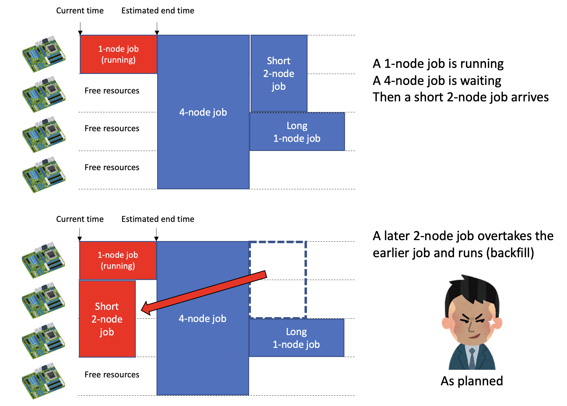
Suppose we have four nodes and allow jobs requesting one through four nodes. A one-node job starts first, followed by submission of a four-node job. The four-node job must wait until every node is free. Another one-node job is then submitted. If the scheduler simply chooses the next runnable job in the queue, it sees three free nodes plus a four-node job and a one-node job, so it runs the one-node job. If one-node and four-node jobs continue to be mixed this way, only the one-node jobs may run and the four-node job may wait forever. Conversely, if the scheduler reserves the next turn for the four-node job while one node is occupied, three nodes remain wasted until that earlier job ends. Backfilling improves this situation.

Jobs state a planned execution time. The scheduler therefore knows when a currently running job is expected to finish. Any job that will finish before that time can safely run ahead of the four-node job. Dispatching jobs in this way is called backfilling.

A supercomputer queue normally has a default maximum execution time. If a job does not specify a requested time, it is usually treated as requesting that maximum. Users often care only whether their job will finish within the maximum and omit the request, thereby requesting the maximum time. But if every job requests the same execution time, no job can be backfilled. Conversely, if a job known to finish quickly requests an accurate short time, backfilling can fit it into gaps and make it more likely to run.

In my experience operating supercomputers, users fall into two extremes: those who submit jobs without thinking about scheduling at all, and those who carefully devise an optimal submission strategy. There is no need to obsess over it. Still, requesting 24 hours for a job that finishes in three, then complaining “It finishes quickly, but I had to wait forever!” when it is slow to start, is not especially reasonable. It may be worth paying at least a little attention to scheduling.

Chained Jobs

As already noted, a shorter requested execution time makes backfilling—and therefore execution—more likely. Even in a queue allowing 24-hour jobs, splitting a calculation into six four-hour jobs may produce results sooner. Each job then writes a checkpoint when it finishes, and the next reads that checkpoint and continues. If the next job starts before the preceding one finishes, it fails. If an early job among the six fails, the remaining jobs should not run either. To support this situation, many schedulers provide job chains or job chaining. This specifies dependencies between jobs, such as “do not run this job until that one finishes” or “do not run the next job if the previous one fails.” The exact syntax depends on the scheduler. Generally, it uses the job ID assigned at submission and submits the next job with a condition such as “run after the job with this ID exits successfully.” For PBS, for example:

To specify the dependency directly in the terminal:

qsub go.sh –W depend=afterok:123456

To put it in the job script:

# PBS -W depend=afterok:123456

Here afterok means “after successful completion.” Besides using backfilling and job chains effectively, you may decide after a run that you want to continue a little longer. Programs submitted to a supercomputer should therefore support checkpoint/restart whenever practical.

Staging

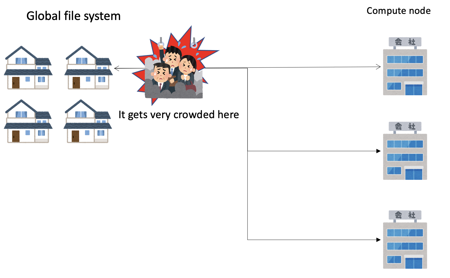
We have already seen that a supercomputer broadly consists of login nodes, compute nodes, and a file system connected by a high-speed network. The file system is mounted on login nodes, where users work. Whether it is also visible from compute nodes depends on the machine’s design. If a file system is visible from both the login nodes and every compute node, it may be called a global file system. Reading and writing it from compute nodes traverses the network, so some network topologies can suffer congestion. In particular, when a large job reads or writes files simultaneously from many nodes, communication links may saturate and lose performance, or contention with other jobs may degrade performance. File I/O then becomes a bottleneck and slows simulations. To prevent this, compute nodes may have small but fast local file systems. A local file system is visible only from its compute node, not even from a login node. Because each compute node has exclusive use, it can read and write quickly. Some systems apparently use SSDs for this local storage.

The local file system attached to each compute node is visible only from that node. Suppose we want to process a large number of files. Each process’s input files must be copied to the local file system attached to the node where that process runs. When processing finishes, the output files must be brought from the local file system back to the global file system before the job ends. But until the job is dispatched, we do not know which compute nodes will run it. The scheduler therefore handles this too.

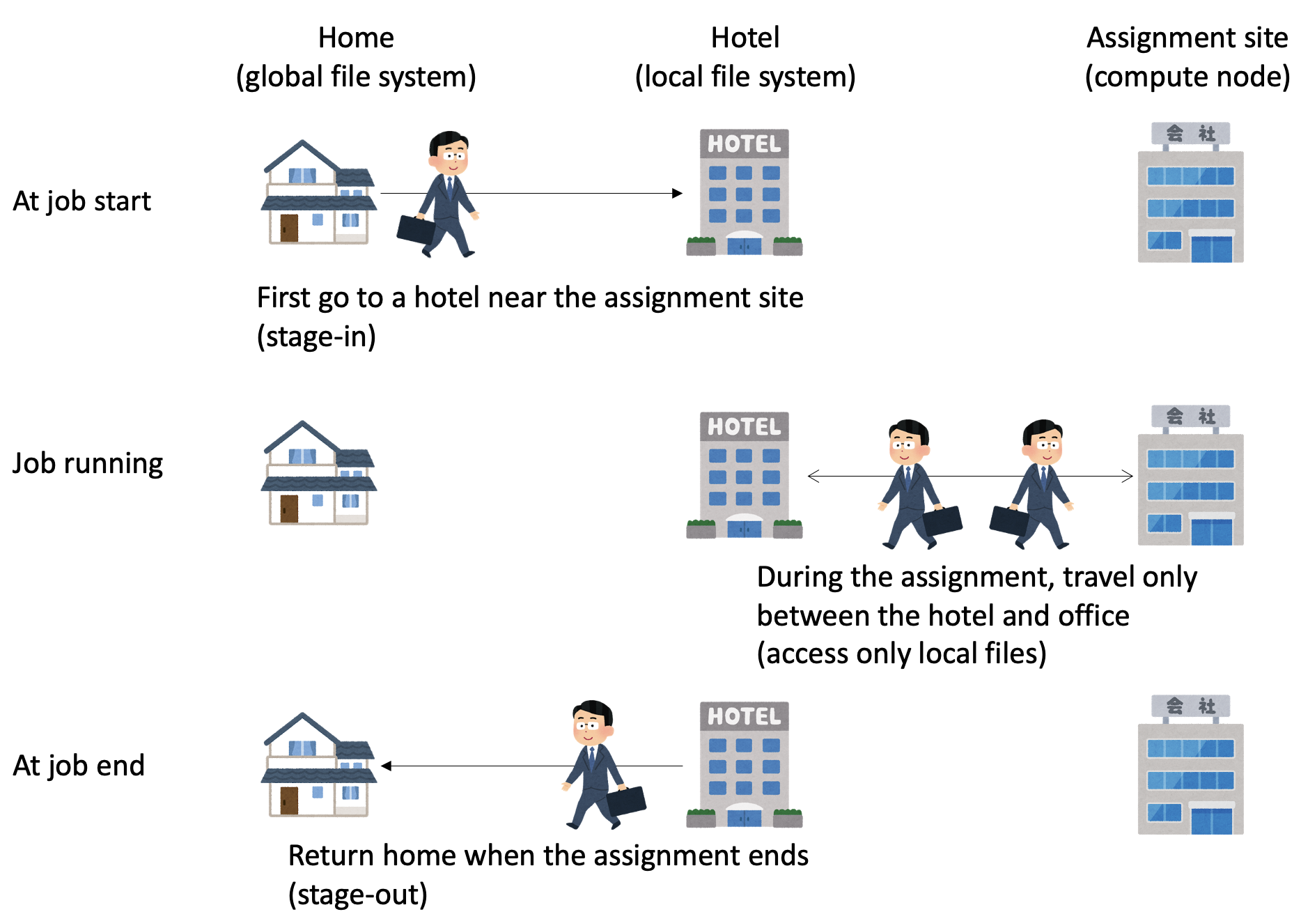
The job script states which files each process needs and which files should ultimately be returned to the global file system. The scheduler reads this information and copies files between the global and local file systems. This operation is called staging. Copying files to local storage before execution is stage-in; retrieving them from local storage after execution is stage-out. Staging methods vary by supercomputer site, so consult the documentation for details. The essential idea is this: if every compute node reads and writes a globally visible file system, network links along the way may become congested. Place files near the compute nodes instead, and transfer them between the compute nodes and global file system only once before and once after the job. By analogy, suppose an employee is assigned for a month to a distant office. Commuting is possible but arduous, so they rent a monthly apartment nearby. Then the long journey is needed only at the beginning and end.

Parallel File Systems

If you never produce an enormous number of files, you may not need to think much about file systems. Nevertheless, a file system is an important component of a supercomputer and worth understanding at least roughly.

What is a file system in the first place? When we open a file by clicking it or display its contents with cat, we rarely consider where or how it is stored on the disk. A hard disk, for example, stores information on circular platters divided into wedge-shaped regions called sectors. Files are stored in units of sectors. To obtain a file’s data, the system must first determine which sectors contain it and then read those sectors. A file may be split across several sectors, in which case all of them must be read. The file system performs this work on our behalf. It manages two main kinds of information: the file data itself, of course, and index information describing which file is located where. This index information is called metadata.

When working in a terminal, you probably run ls routinely. This asks the file system which files are in the current directory. Since no file contents are updated, only metadata is needed. A large supercomputer file system may contain an enormous number of files, making even the index lookup needed to find their locations substantial work. On one supercomputer file system, metadata operations became visibly slower as the total file count grew; an ls command could take several seconds or even more than ten seconds to return. Because a slow ls makes work extremely frustrating, metadata performance is directly tied to user happiness.

A supercomputer connects multiple nodes by a network. If each node had a separate file system, users would need to find out which node ran each submitted job and copy files there, which would be inconvenient. We therefore want a file system visible in common from multiple nodes. NFS has long been widely used for this purpose. It makes a file system attached to one computer visible from another over a network and has a layer that absorbs differences between operating systems and underlying file systems. The provider is called an NFS server, and the machine mounting it over the network is an NFS client. To a client, the remote file system looks like an ordinary directory. Accessing that directory sends requests over the network to the NFS server, allowing files to be searched, created, and deleted.

NFS is convenient for relatively small systems, but becomes extremely slow as the number of clients attached to a server grows. Simultaneous requests from multiple clients keep the server busy, and exhausting network bandwidth creates another bottleneck. Modern supercomputers may have thousands or tens of thousands of nodes; attaching 10,000 nodes to one NFS server is probably impossible. In the past, simultaneous access from many clients could frequently bring down the entire NFS server—although perhaps that was the author’s poor configuration. There is apparently also a parallel standard called pNFS, but the author does not know it well.

In any case, a supercomputer needs a scalable parallel file system that can rapidly serve requests from a very large number of clients. Lustre is now widely used for this purpose. A distinctive feature of Lustre is its separation of servers that manage metadata from those that manage file contents. This allows it to serve the flood of requests from many clients quickly. In the author’s experience, Lustre seems especially fast at responding to metadata queries.

Let us briefly examine how Lustre works. A Metadata Server (MDS) manages the index information for files. The metadata itself is stored in a Metadata Target (MDT). An Object Storage Server (OSS) manages file contents, which are stored in Object Storage Targets (OSTs).

Login and compute nodes are Lustre clients connected to the Lustre system over the network. When a client needs a file’s contents—for example, after cat test.txt—it first asks the MDS where the file is. The MDS replies with the relevant location on an OST. The client then requests the file from that OST, and the OST returns it.

Lustre metadata and read/write performance depend on the server configuration, network, disk controllers, and other factors. Lustre itself does not guarantee fault tolerance, so operators address this by, for example, configuring RAID for MDTs and OSTs. Taking all of this seriously becomes rather involved, and we will not explore it further here.

Finally, readers with access to a Lustre file system can experiment briefly with its client. First move to a directory on a Lustre mount. On most supercomputers, /home is probably Lustre, so your home directory should work. Check with df -T /home to be sure. On a nearby supercomputer, the result looked like this:

$ df -T /home
Filesystem        Type    1K-blocks   Used    Available Use%  Mounted on
path/to/mds:/home lustre  XXXXXXXXXX  YYYYYYY ZZZZZ     PP%   /home

The type of /home is lustre. The numbers and other details have been intentionally obscured. Create an arbitrary directory—for example, temp—and enter it.

mkdir temp
cd temp

Next create a file, say test.txt.

$ touch test.txt
$ ls
test.txt

Now invoke the Lustre client command lfs. Here we will obtain the file ID.

$ lfs path2fid test.txt
[0x20005cf46:0x1794e:0x0]

Lustre manages a file using its File Identifier (FID). In Lustre 2.x, an FID is represented by 128 bits. The first 64 bits are the sequence, the next 32 bits are the object ID, and the final 32 bits are the version. Here, 0x20005cf46 is the sequence, 0x1794e is the object ID, and 0x0 is the version number.

Appending to or renaming the file does not change its FID.

$ echo 1 >> test.txt
$ lfs path2fid test.txt
[0x20005cf46:0x1794e:0x0]

$ mv test.txt test2.txt
$ lfs path2fid test2.txt
[0x20005cf46:0x1794e:0x0]

Deleting and recreating it does change the FID.

$ rm test2.txt; touch test2.txt
$ lfs path2fid test2.txt
[0x20005cf46:0x1799c:0x0]

We will not explore how Lustre uses FIDs to manage files or why it introduced the sequence field. Interested readers should consult the official Lustre documentation.