Day 7: SIMD Vectorization
If you have read this far, thank you for your hard work. If you are starting here, that is fine too. There are three types of parallelization in supercomputer programming: process parallelism, thread parallelism, and data parallelism. We have already discussed process parallelism and thread parallelism, so let us finish by introducing SIMD vectorization, a form of data parallelism.
What Is SIMD?
Section titled “What Is SIMD?”If you are interested in supercomputer programming, you have probably heard the term “SIMD.” SIMD stands for “single instruction, multiple data,” meaning that a single instruction operates on multiple data elements simultaneously. Earlier, we wrote that parallelization can be broadly divided into three types: data parallelism, shared-memory parallelism, and distributed-memory parallelism. SIMD belongs to data parallelism. SIMD instructions are implemented in almost every CPU currently used for general numerical computation. As we will discuss later, SIMD is a technique for performing multiple operations simultaneously in a single cycle, and a CPU’s “theoretical peak performance” refers to its performance when its SIMD capabilities are fully utilized. Therefore, being completely unable to use SIMD is equivalent to reducing peak performance to a fraction of its potential. Let us examine why SIMD is necessary and what SIMD actually is.
A computer is, in essence, a machine that fetches data and instructions from memory, sends them to execution units, and writes the results back to memory. CPU operation is measured in units called “cycles.” It takes several cycles from the time a computation is sent to an execution unit until the result is returned, but modern CPUs use a technique called pipelining to effectively execute one operation per cycle. Since one operation can be executed per cycle, performance can then be improved simply by increasing the “number of cycles per second = clock frequency.”
CPU vendors consequently engaged in fierce competition to increase clock frequencies, but clock frequencies stopped rising in the 2000s. Heat generation caused by leakage current is the main reason, but we will not go into detail here. If one operation can be performed per cycle but the clock frequency can no longer be increased, then improving performance requires performing “multiple operations per cycle.” Several approaches were devised to achieve these “multiple operations per cycle.”
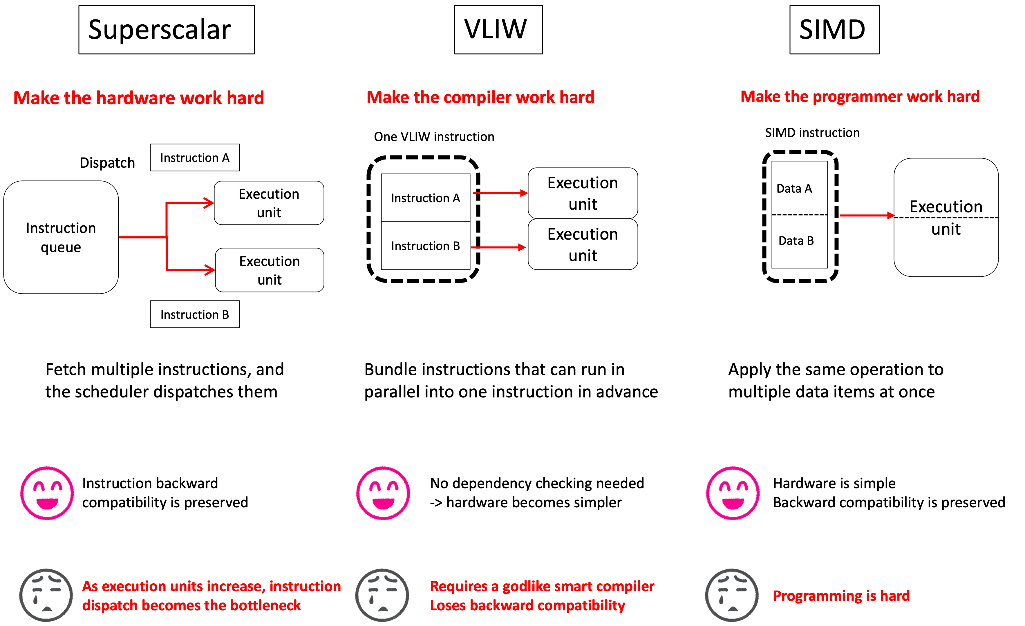
First, one possible approach is simply to increase the number of execution units. The idea is to fetch multiple instructions in one cycle and, if some of them can be executed independently, send them to multiple execution units simultaneously to increase the number of operations per cycle. This is called superscalar execution. Because performance will not improve unless there are instructions that can be executed independently, it is often combined with out-of-order execution. In essence, many instructions are fetched and placed in an instruction queue, and a scheduler examines the queue, selects instructions that can be executed independently, and dispatches them to the execution units.
This approach has the major advantage that it “does not require changing the instruction set.” The hardware automatically finds instructions that can be executed in parallel and executes them simultaneously, so the programmer does not have to do anything. In that sense, superscalar execution is an approach that makes the hardware do the hard work. The disadvantage—or rather, the problem—is that as the number of execution units increases, the effort required for dependency checking grows exponentially. In general, the practical limit is thought to be around four integer operations and two floating-point operations.
Now, the problem with superscalar execution was the complexity of checking instruction dependencies. If only that problem could be solved, one could expect performance to improve simply by adding more execution units. This led to the idea of arranging instructions that can be executed in parallel in advance and feeding them directly to the execution units without checking them. Execution units such as integer units, floating-point units, and memory load/store units are arranged side by side, and all the instructions supplied to them are laid out in advance to form “one instruction.” Because as many instructions as there are execution units capable of operating in parallel are “packed” into a single instruction, the instruction becomes extremely long. This approach is therefore called “Very Long Instruction Word,” or VLIW. In practice, the compiler examines the source code, extracts instructions that can be executed in parallel, and arranges them to maximize parallel execution, thereby creating a single instruction. In that sense, VLIW is an approach that makes the compiler do the hard work.
To gain performance with this approach, a VLIW “instruction” must be filled with useful operations. However, when instructions have many dependencies, fewer execution units can be used simultaneously, so the positions corresponding to idle execution units are filled with “NOPs (no operation).” VLIW was adopted by an architecture called IA-64, jointly developed by Intel and HP, and the Itanium 2 that implemented it saw a fair amount of use in high-end servers and supercomputers. Personally, I like the Itanium 2 (it also has plenty of registers), but this approach requires a “godlike, intelligent compiler” to shine. In general, approaches that demand a “godlike, intelligent compiler” are usually destined to fail. Another serious drawback is that the instruction set is tightly coupled to the execution-unit specifications, resulting in poor backward compatibility. Although VLIW is popular in embedded applications, it is fair to say that it has, for now, become nearly extinct in high-end HPC.
Thus, the approach of “making the hardware do the hard work” had its limits, while the approach of “making the compiler do the hard work” was impractical. The only remaining approach was making the programmer do the hard work. That is SIMD.
Packing different instructions together is difficult. Instead, then, consider packing data rather than instructions. For example, consider the addition C=A+B. This operation “fetches the data A and B, adds them, and writes the result back to memory as C.” Now suppose there are two independent operations, C1 = A1+B1 and C2 = A2+B2. If the data are packed in advance into single registers as A1:A2 and B1:B2, adding them produces a register containing the two packed results C1:C2. A register that packs multiple data elements in this way is called a SIMD register. AVX2, for example, has 256-bit SIMD registers, so four 64-bit double-precision floating-point values can be packed into one register. Independent operations can then be performed on the four packed data elements. The hardware assumes that operations on the packed data have no dependencies. In other words, responsibility for dependencies lies with the programmer. From the hardware’s perspective, it appears that only the “bit width” of the registers and execution units has increased, so the hardware does not become particularly complex. To improve performance, however, programs must be written to make use of SIMD registers.
Improving performance by making use of SIMD registers is commonly called “SIMD vectorization.”
In principle, SIMD vectorization can be performed by the compiler, and in fact, the improvement in the SIMD optimization capabilities of recent compilers is remarkable.
Effective SIMD vectorization, however, often requires changes to data structures. Because it is difficult for a compiler to perform optimizations that involve such global changes, the current situation is that, in general, “SIMD vectorization must be done manually by the programmer.”
Working with SIMD Registers
Section titled “Working with SIMD Registers”SIMD vectorization means improving execution speed by writing code that makes effective use of the SIMD registers implemented in a CPU. To do that, we first need to use SIMD registers. A SIMD register is essentially a variable that can hold multiple data elements at once. Most people reading this probably have a computer with an x86 CPU that supports AVX2. Let us start by using AVX2’s 256-bit registers, the YMM registers. In the following examples, we will use double-precision floating-point variables. Because a double-precision floating-point value is 64 bits, a 256-bit register can hold four such values.
To work with SIMD explicitly, first include x86intrin.h. This makes the _m256d type, which corresponds to a SIMD register, available.
This type treats a 256-bit YMM register as four double-precision floating-point values. To put values into a variable of this type, you can, for example, use the _mm256_set_pd intrinsic.
__m256d v1 = _mm256_set_pd(3.0, 2.0, 1.0, 0.0);This function places values into the register from right to left, starting at the least significant end. In the example above, the double-precision floating-point value 0 goes into the least significant 64 bits, 1 goes into the next 64 bits, and so on.
As noted above, a SIMD register can hold multiple variables simultaneously. In this case, you can think of the _m256d type as being almost equivalent to double [4].
In fact, they can be cast directly. When performing SIMD vectorization, it is useful to prepare a debugging function like this one.
void print256d(__m256d x) { printf("%f %f %f %f\n", x[3], x[2], x[1], x[0]);}You can see that _m256d x can be used directly as double x[4]. Here, x[0] is the least significant element.
Combining this with the earlier assignment gives the following (print.cpp).
#include <cstdio>#include <x86intrin.h>
void print256d(__m256d x) {  printf("%f %f %f %f\n", x[3], x[2], x[1], x[0]);}
int main(void) {  __m256d v1 =  _mm256_set_pd(3.0, 2.0, 1.0, 0.0);  print256d(v1);}
To compile this with g++, you need to tell it that you will be using AVX2.
$ g++ -mavx2 print.cpp$ ./a.out3.000000 2.000000 1.000000 0.000000We can see that the values were correctly assigned to the SIMD register and displayed.
The strength of SIMD registers is that when arithmetic operations are performed between SIMD registers, four computations can be executed simultaneously. Let us verify this.
Let us write a function that simply adds two _m256d values. Arithmetic operators can be applied directly to the _m256d type. You can think of it as something like a class that wraps the double[4] type and overloads its operators.
#include <cstdio>#include <x86intrin.h>
__m256d add(__m256d v1, __m256d v2) {  return v1 + v2;}
Let us look at the assembly. Applying a little optimization makes the assembly easier to read.
g++ -mavx2 -O2 -S add.cppThe assembly looks like this (it has been passed through c++filt, and unnecessary labels have been removed; the same applies below).
add(double vector[4], double vector[4]): vaddpd %ymm1, %ymm0, %ymm0 retvaddpd is an instruction that performs SIMD addition, so we can see that an addition of YMM registers is indeed being invoked.
Let us verify that four elements can actually be added simultaneously (add.cpp).
#include <cstdio>#include <x86intrin.h>
void print256d(__m256d x) {  printf("%f %f %f %f\n", x[3], x[2], x[1], x[0]);}
int main(void) { __m256d v1 = _mm256_set_pd(3.0, 2.0, 1.0, 0.0); __m256d v2 = _mm256_set_pd(7.0, 6.0, 5.0, 4.0); __m256d v3 = v1 + v2; print256d(v3);}$ g++ -mavx2 add.cpp$ ./a.out10.000000 8.000000 6.000000 4.000000We added the vector (0,1,2,3) to the vector (4,5,6,7) and obtained the vector (4,6,8,10).
Because this looks like an operation between vectors, SIMD vectorization is sometimes simply called vectorization. However, unlike the vector products encountered in linear algebra,
note that SIMD multiplication is simply element-wise multiplication. In fact, changing the previous addition to multiplication gives the following (mul.cpp).
#include <cstdio>#include <x86intrin.h>
void print256d(__m256d x) {  printf("%f %f %f %f\n", x[3], x[2], x[1], x[0]);}
int main(void) { __m256d v1 = _mm256_set_pd(3.0, 2.0, 1.0, 0.0); __m256d v2 = _mm256_set_pd(7.0, 6.0, 5.0, 4.0); __m256d v3 = v1 * v2; // Changed to multiplication print256d(v3);}$ g++ -mavx2 mul.cpp$ ./a.out21.000000 12.000000 5.000000 0.000000We can see that it calculated 0*0, 1*5, 2*6, and 3*7, respectively.
Another important aspect of SIMD vectorization is reading and writing data to SIMD registers. We used _mm256_set_pd earlier for debugging, but it is extremely slow. Let us see what it does (setpd.cpp).
#include <x86intrin.h>
__m256d setpd(double a, double b, double c, double d) {  return _mm256_set_pd(d, c, b, a);}
Let us inspect its assembly.
g++ -mavx2 -O2 -S setpd.cppsetpd(double, double, double, double): vunpcklpd %xmm3, %xmm2, %xmm2 vunpcklpd %xmm1, %xmm0, %xmm1 vinsertf128 $0x1, %xmm2, %ymm1, %ymm0 retIt does the following:
- Packs
aandbinto thexmm2register. - Packs
canddinto thexmm0register. - Inserts the value of the
xmm2register into the upper half of theymm0register.
Note that the low 128 bits of the xmm0 and ymm0 registers are shared.
In other words, reading or writing xmm0 also affects the low 128 bits of ymm0.
The example above takes advantage of this fact to produce the desired result: a register containing four packed elements.
Once four elements have been placed in a YMM register, we can calculate with all four simultaneously. Using _mm256_set_pd to pack them, however, requires many memory accesses and delivers poor performance.
There are therefore instructions that load a block of contiguous data from memory into a register or write it back in one operation.
For example, _mm256_load_pd fetches four consecutive double-precision values from a specified pointer and places them in a YMM register. The address indicated by the pointer must be aligned to 32 bytes.
Here is an example (load.cpp).
#include <cstdio>#include <x86intrin.h>
void print256d(__m256d x) {  printf("%f %f %f %f\n", x[3], x[2], x[1], x[0]);}
__attribute__((aligned(32))) double a[] = {0.0, 1.0, 2.0, 3.0, 4.0, 5.0, 6.0, 7.0};
int main(void) {  __m256d v1 = _mm256_load_pd(a);  __m256d v2 = _mm256_load_pd(a + 4);  __m256d v3 = v1 + v2;  print256d(v3);}
Here, __attribute__((aligned(32))) instructs the compiler to align the following data on a 32-byte boundary.
We will not explore memory alignment in detail here; it is enough to remember that the memory being used begins at a suitably positioned boundary.
Specifically, the array’s starting address is divisible by 32. Incorrect memory alignment may reduce performance or cause a run-time SIGSEGV.
Compile and run it as follows.
$ g++ -mavx2 load.cpp$ ./a.out10.000000 8.000000 6.000000 4.000000Let us also see what _mm256_load_pd actually does—that is, which assembly instruction it corresponds to. We will inspect the assembly for the following code (loadasm.cpp).
#include <x86intrin.h>__m256d load(double *a, int index) { return _mm256_load_pd(a + index);}g++ -O2 -mavx2 -S loadasm.cppAs before, we enable a little optimization.
load(double*, int): movslq %esi, %rsi vmovapd (%rdi,%rsi,8), %ymm0 retWe can see that the data is loaded into the ymm0 register with a single vmovapd instruction.
We have looked at loading, and writing data back with _mm256_store_pd works similarly.
This completes the basics of SIMD vectorization. In short, fetch several data values, put them into a SIMD register, perform some calculation in the register, and write them back. Simple, right?
Packing and unpacking scattered data is slow, however, so you should try to load and store contiguous data whenever possible.
When you actually use SIMD, you will encounter questions such as “There is an if statement—what should I do?” or “The memory layout is slightly different from the layout I want in the registers.” A vast number of auxiliary SIMD instructions, such as shuffles, exist to handle these situations. You can learn them as needed. We will now use a simple example to see SIMD vectorization in practice.
Aside: “Assembly Language” or “Assembler Language”?
Section titled “Aside: “Assembly Language” or “Assembler Language”?”Whenever assembly comes up, someone almost invariably insists that assembly language is correct and assembler language is wrong. In almost every case, it is of course fine to understand that an assembler assembles assembly language into machine language. Nevertheless, the expression assembler language does exist. IBM provides the best-known example. IBM has long used the term assembler language. The assembly language that IBM currently supports is IBM High Level Assembler (HLASM), which runs on its System z mainframes. The HLASM manual also uses the term assembler language. Yet the assembly language that ran on System/360, the ancestor of System z, is called IBM Basic Assembly Language (BAL), so the distinction between assembly language and assembler language is subtle. IBM itself describes BAL as Basic Assembler Language, so perhaps IBM calls it Basic Assembler Language while third parties call it Basic Assembly Language.
IBM is not the only example. UAL, an assembly language defined by ARM, stands for Unified Assembler Language. A literal Japanese translation would likewise use “assembler” rather than “assembly.” Yet ARM itself calls assembly language assembly language, so here too the distinction is subtle. In the author’s experience, referring to assembly language simply as “assembler” was once quite common in Japan. People would say, for example, that code written without C or another high-level language was “written entirely in assembler.” Some people still use the word that way today. As an unimportant aside, people writing x86 assembly at the time also seem generally to have called machine language machine code using a transliterated Japanese expression.
To repeat, assembly language appears to be the more common term today, so there is nothing wrong with saying that “an assembler assembles assembly language into machine language.” But when someone says that they “write assembler” or refers to “assembler language,” please remember the circumstances above before reflexively asserting your superiority by correcting them to “assembly language.”
As an aside to the aside, manually translating assembly into machine language is called hand assembly. Older assembly corresponded almost one-to-one with machine language and resembled “machine language with convenient macros,” so hand assembly was not especially difficult. Modern machine language, particularly x86 machine language, has become quite complex, making translation from assembly substantially harder. For more on this subject, see, for example, Introduction to x86-64 Machine Language (Japanese).
A Simple SIMD Example
Section titled “A Simple SIMD Example”Let us now try SIMD vectorization in practice. Consider the following code.
It is a simple loop that adds two one-dimensional arrays (func.cpp).
const int N = 10000;double a[N], b[N], c[N];
void func() {  for (int i = 0; i < N; i++) {    c[i] = a[i] + b[i];  }}
Compiling it normally produces assembly like this:
g++ -O1 -S func.cpp xorl %eax, %eax leaq _a(%rip), %rcx leaq _b(%rip), %rdx leaq _c(%rip), %rsi movsd (%rax,%rcx), %xmm0 addsd (%rax,%rdx), %xmm0 movsd %xmm0, (%rax,%rsi) addq $8, %rax cmpq $80000, %rax jne LBB0_1The addresses of arrays a, b, and c are loaded into %rcx, %rdx, and %rsi, respectively.
The movsd instruction loads the data at a[i] into %xmm0, addsd calculates a[i]+b[i] and stores the result in %xmm0, and another movsd writes it back to the address indicated by c[i].
This is scalar code, but xmm is a 128-bit SIMD register.
For historical reasons, x86 uses the SIMD register xmm for floating-point operations even in scalar code; see the aside below.
Now let us vectorize this loop with AVX2. The basic idea of SIMD vectorization is to unroll a loop, create several independent operations, and execute them simultaneously in SIMD registers. AVX2 SIMD registers are written as ymm. A ymm register is 256 bits wide and can hold four double-precision floating-point values, so we need to:
- unroll the loop by a factor of four;
- load four values from array
ainto aymmregister; - load four values from array
binto aymmregister; - add the two registers; and
- store the resulting register in the appropriate positions of array
c.
That completes the SIMD vectorization. It will be quicker to look at the code (func_simd.cpp).
#include <x86intrin.h>void func_simd() { for (int i = 0; i < N; i += 4) { __m256d va = _mm256_load_pd(&(a[i])); __m256d vb = _mm256_load_pd(&(b[i])); __m256d vc = va + vb; _mm256_store_pd(&(c[i]), vc); }}As we saw earlier, _mm256_load_pd loads four consecutive values, while _mm256_store_pd stores the contents of a SIMD register in memory.
Let us compile this code and inspect the assembly.
g++ -O1 -mavx2 -S func_simd.cpp xorl %eax, %eax leaq _a(%rip), %rcx leaq _b(%rip), %rdx leaq _c(%rip), %rsi xorl %edi, %ediLBB0_1: vmovupd (%rax,%rcx), %ymm0 # (a[i],a[i+1],a[i+2],a[i+3]) -> ymm0 vaddpd (%rax,%rdx), %ymm0, %ymm0 # ymm0 + (b[i],b[i+1],b[i+2],b[i+3]) -> ymm 0 vmovupd %ymm0, (%rax,%rsi) # ymm0 -> (c[i],c[i+1],c[i+2],c[i+3]) addq $4, %rdi # i += 4 addq $32, %rax cmpq $10000, %rdi jb LBB0_1The assembly corresponds almost directly to the source, so it should not be difficult to understand even if you are unfamiliar with assembly.
As before, the addresses of the arrays are loaded into %rcx, %rdx, and %rsi.
Where the original code used movsd to copy data into an xmm register, this version uses vmovupd to copy data into a ymm register.
The Intel Intrinsics Guide is a useful reference for finding which intrinsic corresponds to which SIMD instruction.
To be safe, let us check that this code calculates the correct result.
We generate arbitrary random numbers and store them in arrays a[N] and b[N], while also storing the expected answers in ans[N].
int main() { std::mt19937 mt; std::uniform_real_distribution<double> ud(0.0, 1.0); for (int i = 0; i < N; i++) { a[i] = ud(mt); b[i] = ud(mt); ans[i] = a[i] + b[i]; } check(func, "scalar"); check(func_simd, "vector");}Comparing two double-precision floating-point values for equality has various subtleties, so let us compare them byte by byte.
Here, arrays c[N] and ans[N] are cast to unsigned char and compared.
void check(void(*pfunc)(), const char *type) { pfunc(); unsigned char *x = (unsigned char *)c; unsigned char *y = (unsigned char *)ans; bool valid = true; for (int i = 0; i < 8 * N; i++) { if (x[i] != y[i]) { valid = false; break; } } if (valid) { printf("%s is OK\n", type); } else { printf("%s is NG\n", type); }}Save the complete code as simdcheck.cpp and run it.
#include <cstdio>#include <random>#include <algorithm>#include <x86intrin.h>
const int N = 10000;
double a[N], b[N], c[N];double ans[N];
void check(void(*pfunc)(), const char *type) {  pfunc();  unsigned char *x = (unsigned char *)c;  unsigned char *y = (unsigned char *)ans;  bool valid = true;  for (int i = 0; i < 8 * N; i++) {    if (x[i] != y[i]) {      valid = false;      break;    }  }  if (valid) {    printf("%s is OK\n", type);  } else {    printf("%s is NG\n", type);  }}
void func() {  for (int i = 0; i < N; i++) {    c[i] = a[i] + b[i];  }}
void func_simd() {  for (int i = 0; i < N; i += 4) {    __m256d va = _mm256_load_pd(&(a[i]));    __m256d vb = _mm256_load_pd(&(b[i]));    __m256d vc = va + vb;    _mm256_store_pd(&(c[i]), vc);  }}
int main() {  std::mt19937 mt;  std::uniform_real_distribution<double> ud(0.0, 1.0);  for (int i = 0; i < N; i++) {    a[i] = ud(mt);    b[i] = ud(mt);    ans[i] = a[i] + b[i];  }  check(func, "scalar");  check(func_simd, "vector");}
Let us actually run the test.
$ g++ -mavx2 -O3 simdcheck.cpp$ ./a.outscalar is OKvector is OKThe calculations appear to be correct.
A compiler can vectorize code this simple for us. The question, then, is how to determine whether the compiler actually did so.
One method is to inspect the compiler’s optimization report. With the Intel compiler, the -qopt-report option produces such a report.
$ icpc -march=core-avx2 -O2 -c -qopt-report -qopt-report-file=report.txt func.cpp$ cat report.txtIntel(R) Advisor can now assist with vectorization and show optimization report messages with your source code.(snip)LOOP BEGIN at func.cpp(5,3) remark #15300: LOOP WAS VECTORIZEDLOOP ENDThe actual report contains considerably more clutter, but the final LOOP WAS VECTORIZED tells us that vectorization succeeded.
It gives us no idea, however, how the compiler vectorized the loop. Let us increase the optimization-report level with -qopt-report=5.
$ icpc -march=core-avx2 -O2 -c -qopt-report=5 -qopt-report-file=report5.txt func.cpp$ cat report5.txtIntel(R) Advisor can now assist with vectorization and show optimization report messages with your source code.(snip)LOOP BEGIN at func.cpp(5,3) remark #15388: vectorization support: reference c has aligned access [ func.cpp(6,5) ] remark #15388: vectorization support: reference a has aligned access [ func.cpp(6,5) ] remark #15388: vectorization support: reference b has aligned access [ func.cpp(6,5) ] remark #15305: vectorization support: vector length 4 remark #15399: vectorization support: unroll factor set to 4 remark #15300: LOOP WAS VECTORIZED remark #15448: unmasked aligned unit stride loads: 2 remark #15449: unmasked aligned unit stride stores: 1 remark #15475: --- begin vector loop cost summary --- remark #15476: scalar loop cost: 6 remark #15477: vector loop cost: 1.250 remark #15478: estimated potential speedup: 4.800 remark #15488: --- end vector loop cost summary --- remark #25015: Estimate of max trip count of loop=625LOOP ENDThe report tells us the following:
- SIMD vectorization uses
ymmregisters (vector length 4); - the loop was unrolled by a factor of four (
unroll factor set to 4); - the scalar-loop cost was estimated as 6 (
scalar loop cost: 6); - the vector-loop cost was estimated as 1.250 (
vector loop cost: 1.250); and - vectorization was estimated to provide a 4.8-fold speedup (
estimated potential speedup: 4.800).
In a situation like this, though, it is quicker to look at the assembly.
icpc -march=core-avx2 -O2 -S func.cppHere is the assembly produced by the compiler, with its instructions rearranged slightly by hand.
xorl %eax, %eax..B1.2: lea (,%rax,8), %rdx vmovupd a(,%rax,8), %ymm0 vmovupd 32+a(,%rax,8), %ymm2 vmovupd 64+a(,%rax,8), %ymm4 vmovupd 96+a(,%rax,8), %ymm6 vaddpd b(,%rax,8), %ymm0, %ymm1 vaddpd 32+b(,%rax,8), %ymm2, %ymm3 vaddpd 64+b(,%rax,8), %ymm4, %ymm5 vaddpd 96+b(,%rax,8), %ymm6, %ymm7 vmovupd %ymm1, c(%rdx) vmovupd %ymm3, 32+c(%rdx) vmovupd %ymm5, 64+c(%rdx) vmovupd %ymm7, 96+c(%rdx) addq $16, %rax cmpq $10000, %rax jb ..B1.2We manually unrolled the loop by a factor of four for SIMD vectorization earlier; we can see that the compiler has unrolled it by another factor of four.
I can state this categorically: when investigating compiler optimization of this kind, reading the assembly is always faster than staring at the compiler’s optimization report.
Many people brace themselves when they hear “read the assembly,” but there are not that many instructions used for SIMD vectorization anyway. At the very least, merely checking which kind of registers appear tells you whether vectorization worked properly.
Even if you do not understand algorithms such as loop unrolling, seeing assembly full of xmm registers tells you that it has not been vectorized—or not very much. ymm registers indicate SIMD vectorization with AVX/AVX2, while zmm registers indicate AVX-512. The appearance of vmovupd suggests smooth copying from memory, and vaddpd shows that addition is actually being done with SIMD. This level of understanding is often enough in practice.
If you keep reading assembly in this way, you may eventually overcome your instinctive dislike of it and gradually begin to understand what the compiler was thinking.
Aside: How x86 Handles Floating-Point Operations
Section titled “Aside: How x86 Handles Floating-Point Operations”Floating-point operations are essential in numerical computing. A floating-point number is represented by 32 bits in single precision or 64 bits in double precision. The representation is defined by the IEEE 754 standard. A CPU performs calculations in registers, and it generally provides separate general-purpose registers for integer operations and floating-point registers for floating-point operations. CPUs that support double-precision operations commonly have 64-bit floating-point registers. x86 is an exception: it has no 64-bit floating-point register. Instead, it uses 128-bit SIMD registers called XMM registers even for ordinary floating-point calculations. This is the result of the history of floating-point support on x86.
Originally, x86 could not perform floating-point operations in hardware. Floating-point calculations therefore had to be emulated in software using general-purpose registers, which was extremely slow. The x87 coprocessor was introduced to provide floating-point support.
A coprocessor is an external device placed near the CPU to extend its functionality. When the CPU encounters an instruction supported by the coprocessor, it delegates the operation to that device.
From the user’s perspective, the CPU’s instruction set appears to have been extended. The x87 coprocessor is an 80-bit machine. Whether a value is single precision (32 bits) or double precision (64 bits), it is first converted internally to 80 bits for calculation, after which the result is converted back to single or double precision. A long double, by contrast, is calculated directly as an 80-bit value with no conversion. This is why long double is 80 bits on x86 processors.
The x87 coprocessor evolved along with x86. The Intel 8086 was paired with the Intel 8087, the 80186 with the 80187, the 80286 with the 80287, and so forth. The family is called x87 in the same manner as x86. For some time, x87 remained an external coprocessor, but starting with the 80486 it was integrated into the CPU.
Floating-point computation also has another historical thread: SIMD. As CPU performance increased, demand grew for faster audio and video encoding and decoding, 3D processing, and similar workloads. In response, AMD announced the 3DNow! SIMD instruction-set extension. It extended Intel’s MMX and used 64-bit MMX registers to perform two single-precision floating-point operations simultaneously. Intel subsequently introduced the SSE SIMD instruction-set extension, along with 128-bit XMM registers. At first, XMM registers could handle only single-precision operations, but SSE2 added support for double precision. AMD began using XMM registers by default for double-precision calculations, and Intel apparently followed later, although the author is not familiar with the exact chronology.
Thus, x86 has the 80-bit floating-point registers introduced with x87 and the 128-bit XMM registers introduced with SSE, but an “ordinary” 64-bit floating-point register was never introduced. Modern x86 uses the low 64 bits of an XMM SIMD register even for everyday, non-SIMD double-precision operations.
SIMD instruction-set extensions subsequently continued to develop through AVX, AVX2, and AVX-512, increasing SIMD widths to 256 and 512 bits. The SIMD registers expanded accordingly to YMM and ZMM. The low 128 bits of YMM are XMM, and the low 256 bits of ZMM are YMM, much as the general-purpose registers AX, EAX, and RAX have a containment relationship.
A More Practical SIMD Example
Section titled “A More Practical SIMD Example”The SIMD vectorization discussed above was extremely simple and could be performed automatically by the compiler. In general, however, SIMD can involve such complications as shuffling values within registers and choosing appropriate data structures. For dedicated SIMD enthusiasts who want something more substantial, let us examine a slightly more practical example.
Consider the motion of charged particles in a magnetic field. Let the magnetic-field vector be , the velocity vector , and the position vector . For simplicity, use a system of units in which the elementary charge, mass, and speed of light are all 1. The equations of motion are
Writing the time derivative of velocity component by component gives
In a magnetic field, a charged particle moves uniformly in a straight line parallel to the field and in a circle perpendicular to it. Its resulting trajectory is a helix, as shown below.
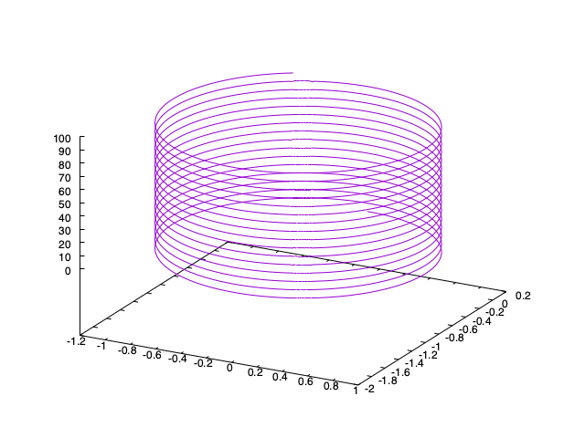
Let us simulate charged particles scattered through a magnetic field pointing in an arbitrary direction, each with an initial velocity in a random direction. We also neglect interactions between particles. Since this is a three-dimensional simulation, represent a three-dimensional vector with a structure.
struct vec { double x, y, z;};Let the number of particles be N, and store their position and velocity vectors in arrays of structures.
const int N = 100000;vec r[N], v[N];Time evolution using the first-order Euler method can then be written as follows.
void calc_euler() { for (int i = 0; i < N; i++) { double px = v[i].y * BZ - v[i].z * BY; double py = v[i].z * BX - v[i].x * BZ; double pz = v[i].x * BY - v[i].y * BX; v[i].x += px * dt; v[i].y += py * dt; v[i].z += pz * dt; r[i].x = r[i].x + v[i].x * dt; r[i].y = r[i].y + v[i].y * dt; r[i].z = r[i].z + v[i].z * dt; }}As is well known, however, the first-order Euler method is highly inaccurate. If you have studied physics, you should know that a magnetic field does no work on a charged particle. The total energy must therefore be conserved. Since there are no particle-particle interactions, the energy consists solely of kinetic energy.
double energy(void) { double e = 0.0; for (int i = 0; i < N; i++) { e += v[i].x * v[i].x; e += v[i].y * v[i].y; e += v[i].z * v[i].z; } return e * 0.5 / static_cast<double>(N);}It is convenient to express quantities such as kinetic energy per particle—that is, as an average—so that they do not depend on the number of particles. The time evolution can be written as follows.
init(); double t = 0.0; for (int i = 0; i < 10000; i++) { calc_euler(); t += dt; if ((i % 1000) == 0) { std::cout << t << " " << energy() << std::endl; } }The average energy evolves as shown below.
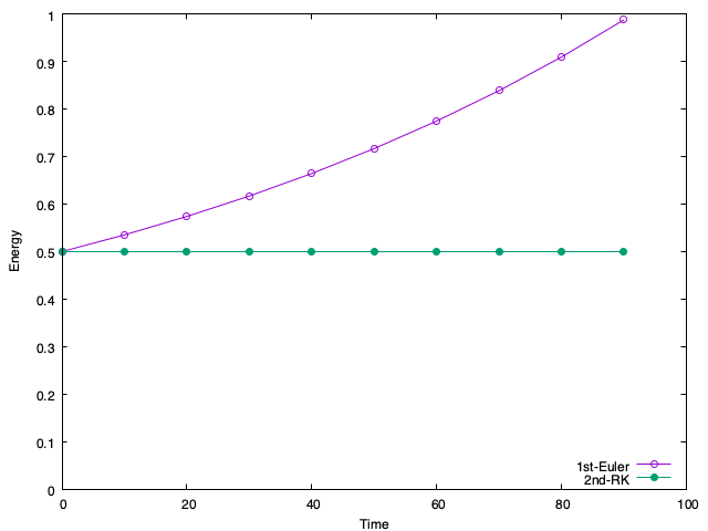
The points labeled “1st-Euler” are from the first-order Euler method. The energy, which should be conserved, steadily increases.
Many numerical integration methods offer greater accuracy; here we will use the simple second-order Runge-Kutta (RK) method.
void calc_rk2() { for (int i = 0; i < N; i++) { double px = v[i].y * BZ - v[i].z * BY; double py = v[i].z * BX - v[i].x * BZ; double pz = v[i].x * BY - v[i].y * BX; double vcx = v[i].x + px * dt * 0.5; double vcy = v[i].y + py * dt * 0.5; double vcz = v[i].z + pz * dt * 0.5; double px2 = vcy * BZ - vcz * BY; double py2 = vcz * BX - vcx * BZ; double pz2 = vcx * BY - vcy * BX; v[i].x += px2 * dt; v[i].y += py2 * dt; v[i].z += pz2 * dt; r[i].x += v[i].x * dt; r[i].y += v[i].y * dt; r[i].z += v[i].z * dt; }}Second-order RK first uses a first-order Euler step to advance the system provisionally by half a time step, evaluates the time derivative again at that intermediate point, and uses that derivative to advance from the current time. “Runge-Kutta” commonly refers to the fourth-order method, but we take the shortcut of using second order here. We also leave the position update as first-order Euler because it is unchanged either way.
The points labeled “2nd-RK” in the preceding figure show the energy calculated this way. It is conserved very accurately. Let us SIMD-vectorize the function calc_rk2.
We previously noted that fetching contiguous data is important for SIMD vectorization. Since we are using YMM registers, we want to load four elements at a time. Each particle in this three-dimensional simulation, however, has a three-element velocity and a three-element position. We must address this first.
Specifically, extend each three-element vector to four elements.
struct vec { double x, y, z, w; // Add w};This allows a particle’s entire velocity to be loaded into a register with one instruction.
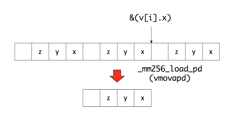
In the figure, the pointer &v[i].x refers to the first element of particle ‘s velocity vector, so
// vv <- (w,z,y,x)__m256d vv = _mm256_load_pd((double *)(&(v[i].x)));loads the three useful values into a register at once, with one element wasted.
Next, we want to calculate the derivative from the data in the register, but its current arrangement does not directly form a cross product. The desired calculation is
double px = v[i].y * BZ - v[i].z * BY; double py = v[i].z * BX - v[i].x * BZ; double pz = v[i].x * BY - v[i].y * BX;To perform this calculation while keeping the values in registers, we must rearrange (x,y,z,w) into (y,z,x,w). SIMD provides shuffle instructions for rearranging elements within a register. For details, see the AVX Double-Precision Shuffle Instruction Cheat Sheet (in Japanese). The output order is encoded as a base-4 number. For example, to rearrange a register from (0,1,2,3) to (1,2,0,3), use
const int im_yzx = 64 * 3 + 16 * 0 + 4 * 2 + 1 * 1;as the argument. Note that this value is 3021 in base 4. Then write
// (w,x,z,y) <- (w,z,y,x) __m256d vv_yzx = _mm256_permute4x64_pd(vv, im_yzx);Note: It is easy to become confused about which side contains the lower-order elements. Registers are conventionally written with lower bits on the right, giving the order (w,z,y,x). Mathematical vectors, on the other hand, conventionally place the first component on the left, inviting the notation (x,y,z,w). Keep this distinction in mind when reading the discussion.
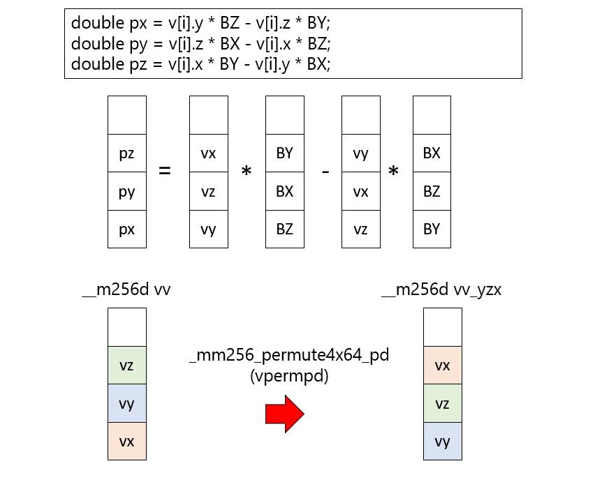
We can now rearrange register contents as needed and add, multiply, or subtract them. For the magnetic field, only the vector arrangements (z,x,y,0) and (y,z,x,0) are needed, so define them in advance.
__m256d vb_zxy = _mm256_set_pd(0.0, BY, BX, BZ); __m256d vb_yzx = _mm256_set_pd(0.0, BX, BZ, BY);The vertical vector calculation shown in the center of the preceding figure becomes the following single line in code:
__m256d vp = vv_yzx * vb_zxy - vv_zxy * vb_yzx;This is why SIMD operations are called vector operations.
It is straightforward to use this to obtain the derivative at the midpoint, and then to update the velocity using that derivative.
Suppose the velocity vector is stored in __m256d vv. Since this is a register, it must be written back to memory. As with loading, store it at the location pointed to by &v[i].x.
// (w,z,y,z) -> v[i]_mm256_store_pd((double *)(&(v[i].x)), vv);Update the position similarly using the new velocity:
__m256d vr = _mm256_load_pd((double *)(&(r[i].x))); vr += vv * vdt; _mm256_store_pd((double *)(&(r[i].x)), vr);Combining these steps gives the following SIMD version of the time-evolution routine.
void calc_rk2_simd() { __m256d vb_zxy = _mm256_set_pd(0.0, BY, BX, BZ); __m256d vb_yzx = _mm256_set_pd(0.0, BX, BZ, BY); __m256d vdt = _mm256_set_pd(0.0, dt, dt, dt); __m256d vdt_h = _mm256_set_pd(0.0, dt * 0.5, dt * 0.5, dt * 0.5); const int im_yzx = 64 * 3 + 16 * 0 + 4 * 2 + 1 * 1; const int im_zxy = 64 * 3 + 16 * 1 + 4 * 0 + 1 * 2; for (int i = 0; i < N; i++) { __m256d vv = _mm256_load_pd((double *)(&(v[i].x))); __m256d vr = _mm256_load_pd((double *)(&(r[i].x))); __m256d vv_yzx = _mm256_permute4x64_pd(vv, im_yzx); __m256d vv_zxy = _mm256_permute4x64_pd(vv, im_zxy); __m256d vp = vv_yzx * vb_zxy - vv_zxy * vb_yzx; __m256d vc = vv + vp * vdt_h; __m256d vp_yzx = _mm256_permute4x64_pd(vc, im_yzx); __m256d vp_zxy = _mm256_permute4x64_pd(vc, im_zxy); __m256d vp2 = vp_yzx * vb_zxy - vp_zxy * vb_yzx; vv += vp2 * vdt; vr += vv * vdt; _mm256_store_pd((double *)(&(v[i].x)), vv); _mm256_store_pd((double *)(&(r[i].x)), vr); }}The routine grew only from 19 lines to 23, so it is not especially complicated. The four additional lines merely construct the magnetic-field vectors and prepare the shuffle indices. Writing this routine all at once would invite bugs, but it is not difficult if you vectorize incrementally within the serial code and verify at every step that the SIMD registers match the serial routine’s values.
Although the routine is now vectorized, neither the operation order nor anything else has changed, so it should match the serial code exactly, including rounding errors. To verify this, dump the position vectors after time evolution.
void dump() { for (int i = 0; i < N; i++) { std::cout << r[i].x << " "; std::cout << r[i].y << " "; std::cout << r[i].z << std::endl; }}Dump the coordinates after time evolution and compare the results. Let mag.cpp be the serial version and mag_simd.cpp the SIMD version. Compile, run, and compare them as follows.
$ g++ -std=c++11 -O3 -mavx2 -mfma mag.cpp -o a.out$ g++ -std=c++11 -O3 -mavx2 -mfma mag_simd.cpp -o b.out$ time ./a.out > a.txt./a.out > a.txt  4.58s user 0.27s system 99% cpu 4.876 total
$ time ./b.out > b.txt./b.out > b.txt  2.54s user 0.29s system 99% cpu 2.849 total
$ diff a.txt b.txt # Results match
Execution time improves from 4.58 s to 2.54 s, and the results match.
It is too early, however, to look at this result and conclude that SIMD worked reasonably well. The preceding data structure was an array of structures, known as an Array of Structures (AoS). The same data can instead be represented as separate arrays:
double rx[N], ry[N], rz[N];double vx[N], vy[N], vz[N];Although these arrays are not literally wrapped in a structure here, this layout is called a Structure of Arrays (SoA). Whether AoS or SoA is preferable depends on the situation, but SoA often performs better for SIMD vectorization.
mag_soa.cpp implements exactly the same calculation as the preceding serial AoS code, but uses an SoA layout. Its time-evolution routine, for example, is as follows.
void calc_rk2() { for (int i = 0; i < N; i++) { double px = vy[i] * BZ - vz[i] * BY; double py = vz[i] * BX - vx[i] * BZ; double pz = vx[i] * BY - vy[i] * BX; double vcx = vx[i] + px * dt * 0.5; double vcy = vy[i] + py * dt * 0.5; double vcz = vz[i] + pz * dt * 0.5; double px2 = vcy * BZ - vcz * BY; double py2 = vcz * BX - vcx * BZ; double pz2 = vcx * BY - vcy * BX; vx[i] += px2 * dt; vy[i] += py2 * dt; vz[i] += pz2 * dt; rx[i] = rx[i] + vx[i] * dt; ry[i] = ry[i] + vy[i] * dt; rz[i] = rz[i] + vz[i] * dt; }}The only apparent change is that expressions such as v[i].x become vx[i]; otherwise it is identical. Run this version and compare its result as well.
$ g++ -std=c++11 -O3 -mavx2 -mfma mag_soa.cpp -o c.out$ time ./c.out > c.txt./c.out > c.txt  1.20s user 0.28s system 98% cpu 1.493 total
$ diff a.txt c.txt # Results match
Compared with the manually vectorized version, execution improves by more than a factor of two, from 2.54 s to 1.20 s. It is nearly four times faster than the original 4.58-second serial code. In other words, compiler auto-vectorization made this code four times faster, achieving nearly ideal SIMD performance.
The compiler actually emits the following code.
L10: vmovapd (%rdi,%rax), %ymm0 vmovapd (%r9,%rax), %ymm11 vmovapd (%r8,%rax), %ymm10 vmulpd %ymm7, %ymm0, %ymm2 vmulpd %ymm11, %ymm5, %ymm1 vfmsub231pd %ymm6, %ymm0, %ymm1 vmulpd %ymm4, %ymm1, %ymm1 vmulpd %ymm10, %ymm6, %ymm3 vfmadd132pd %ymm8, %ymm10, %ymm1 vfmsub231pd %ymm11, %ymm7, %ymm3 vfmsub231pd %ymm10, %ymm5, %ymm2 vmulpd %ymm4, %ymm3, %ymm3 vmulpd %ymm4, %ymm2, %ymm2 vfmadd132pd %ymm8, %ymm0, %ymm3 vfmadd132pd %ymm8, %ymm11, %ymm2 vmulpd %ymm6, %ymm1, %ymm9 vfmsub231pd %ymm7, %ymm2, %ymm9 vmulpd %ymm5, %ymm2, %ymm2 vfmadd132pd %ymm4, %ymm0, %ymm9 vfmsub231pd %ymm6, %ymm3, %ymm2 vmovapd %ymm9, (%rdi,%rax) vfmadd132pd %ymm4, %ymm10, %ymm2 vfmadd213pd (%rsi,%rax), %ymm4, %ymm9 vmovapd %ymm2, (%r8,%rax) vmulpd %ymm7, %ymm3, %ymm0 vfmadd213pd (%rdx,%rax), %ymm4, %ymm2 vfmsub231pd %ymm5, %ymm1, %ymm0 vmovapd %ymm9, (%rsi,%rax) vfmadd132pd %ymm4, %ymm11, %ymm0 vmovapd %ymm2, (%rdx,%rax) vmovapd %ymm0, (%r9,%rax) vfmadd213pd (%rcx,%rax), %ymm4, %ymm0 vmovapd %ymm0, (%rcx,%rax) addq $32, %rax cmpq $800000, %rax jne L10This is only the innermost loop, but it is filled with ymm registers and is clearly vectorized ideally. There are no shuffle instructions at all. The compiler simply unrolls the loop fourfold and calculates with data arranged in each register as (x1, x2, x3, x4). The loop counter is %rax; it increases by 32 each time and stops at 800000, so the loop executes 25,000 iterations.
For comparison, the assembly for the manually vectorized loop is shown below.
L13: vmovapd (%rax), %ymm2 addq $32, %rax addq $32, %rdx vpermpd $201, %ymm2, %ymm0 vpermpd $210, %ymm2, %ymm1 vmulpd %ymm3, %ymm1, %ymm1 vfmsub132pd %ymm4, %ymm1, %ymm0 vfmadd132pd %ymm6, %ymm2, %ymm0 vpermpd $201, %ymm0, %ymm1 vpermpd $210, %ymm0, %ymm0 vmulpd %ymm3, %ymm0, %ymm0 vfmsub231pd %ymm4, %ymm1, %ymm0 vfmadd132pd %ymm5, %ymm2, %ymm0 vmovapd %ymm0, -32(%rax) vmovapd %ymm0, %ymm1 vfmadd213pd -32(%rdx), %ymm5, %ymm1 vmovapd %ymm1, -32(%rdx) cmpq %rcx, %rax jne L13vpermpd is the shuffle instruction. Although this loop body is considerably smaller, it executes 100,000 times and cannot beat the compiler-vectorized routine, which executes only 25,000 times. Roughly speaking, its loop body costs half as much but runs four times as often, making it twice as slow overall.
As this example demonstrates, even if you painstakingly vectorize existing code in place and make it faster, changing the data layout may let the compiler auto-vectorize it effortlessly and outperform your work. SIMD vectorization often entails global changes to data structures. The AoS version mag.cpp and SoA version mag_soa.cpp perform exactly the same calculation, yet the latter is a complete rewrite. That is manageable for this short program, but with 100,000 lines of code one cannot casually say, “SoA is faster after all, so rewrite everything!” Different devices also favor different layouts. It is quite common, for example, for AoS to be faster on a CPU while SoA is faster on a GPGPU. In such cases one may consider converting between AoS and SoA before entering a hotspot routine, but the conversion introduces its own overhead and further complications.
Although this discussion has described many complications, readers who actually work through the examples will probably agree that SIMD vectorization is simple in principle. MPI and SIMD are alike: many considerations make them tedious, but the operations themselves are straightforward rather than difficult. We used shuffle instructions here, but SIMD also offers masks, gather/scatter, pack/unpack, and many other operations. If you find yourself wishing for a particular instruction, it usually exists; you then call the corresponding intrinsic. In short, you only have to implement it.
There is, however, an important difference. Implementing MPI gives you a parallel calculation, and increasing the computation per process can be expected to improve parallel efficiency almost without limit. SIMD vectorization may or may not improve performance, and leaving the work to the compiler can be faster than intervening poorly. For completely unvectorized code, the theoretical SIMD gain is only about fourfold at 256 bits and eightfold even at 512 bits; in practice, achieving half of that is already a good result. SIMD optimization is enjoyable, but in the author’s experience it is debatable whether the effort and cost are worthwhile.