Day 4: Non-Trivial Parallelism with Domain Decomposition

So far, we have dealt with embarrassingly parallel computing. Because it requires almost no communication and offers high parallel efficiency, it makes extremely effective use of computing resources. Since we have access to a supercomputer, however, let us now tackle genuinely non-trivial parallelism involving communication.

Non-Trivial Parallelism

We have already said that a supercomputer is a collection of nodes, and that a node is essentially the same as a PC. But merely connecting many ordinary PCs does not necessarily create a supercomputer: its network and reliability are crucial. The embarrassingly parallel computing discussed so far requires neither.

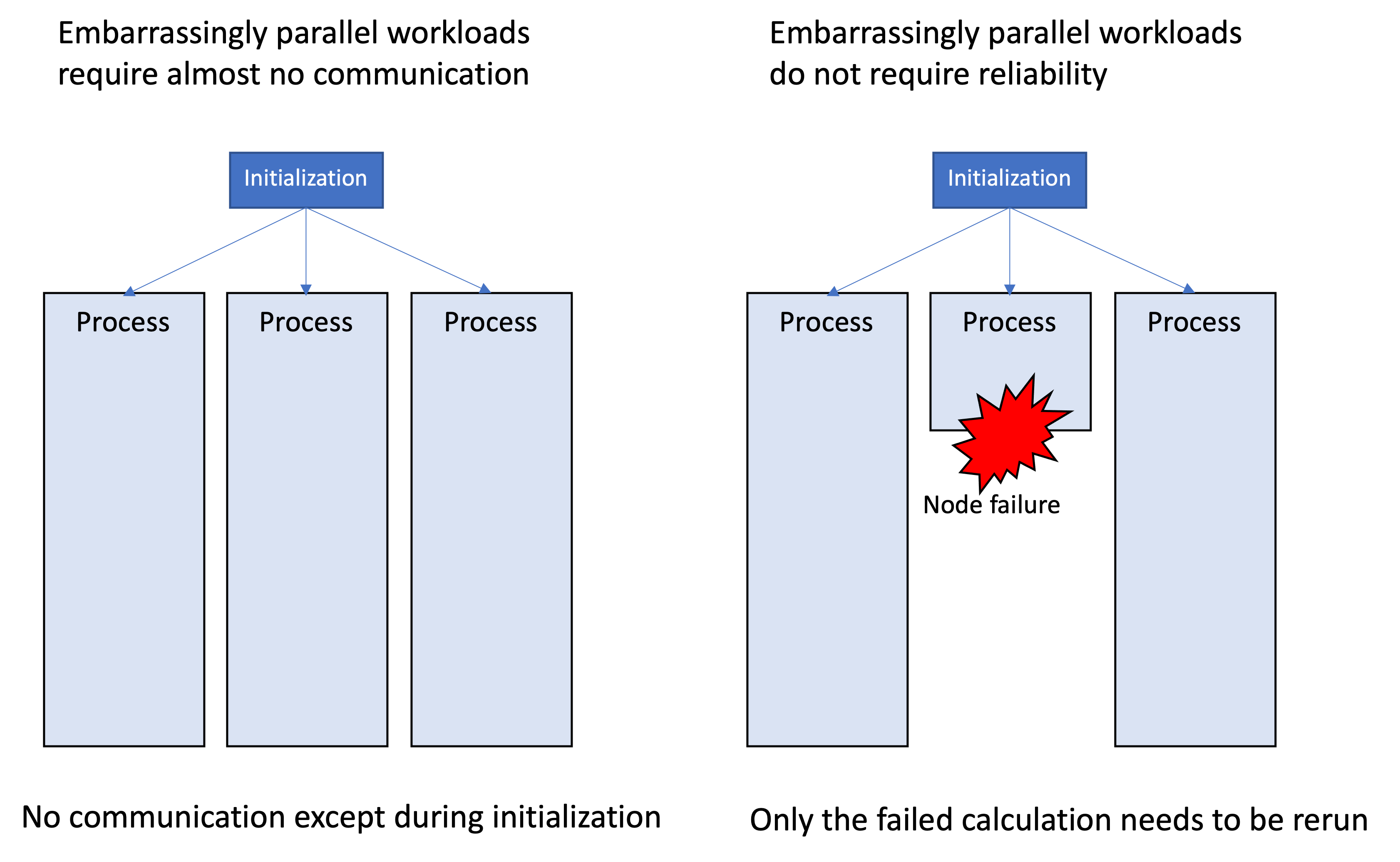
In parameter parallelism, communication is unnecessary after the initial distribution of parameter values to processes; the results can simply be written to files when the calculations finish. The nodes therefore need not be connected by a high-speed network, and ordinary Ethernet is entirely adequate. Large non-trivial parallel calculations demand high reliability, but embarrassingly parallel work does not. If a node fails during a run, only that node’s calculation needs to be repeated. Thus, although embarrassingly parallel computing uses computational resources as efficiently as possible, it makes no use of two defining properties of a supercomputer: its network and reliability. If this is your main workload, a PC cluster made by connecting many ordinary computers is perfectly sufficient.

Embarrassingly parallel or otherwise, using a supercomputer to produce good scientific results is entirely worthwhile. Still, since we have one, we would like to make use of more of what makes it a supercomputer. Let us therefore attempt non-trivial parallelism, which requires both network performance and reliability.

Unlike embarrassingly parallel programs, non-trivial parallel programs require frequent communication. Scientific computing often involves an iterative calculation such as time evolution, and meaningful parallelization may require communication at every step. Such calculations fall broadly into two types: those that communicate with every participating node at each step, and those that communicate only with logically nearby nodes.

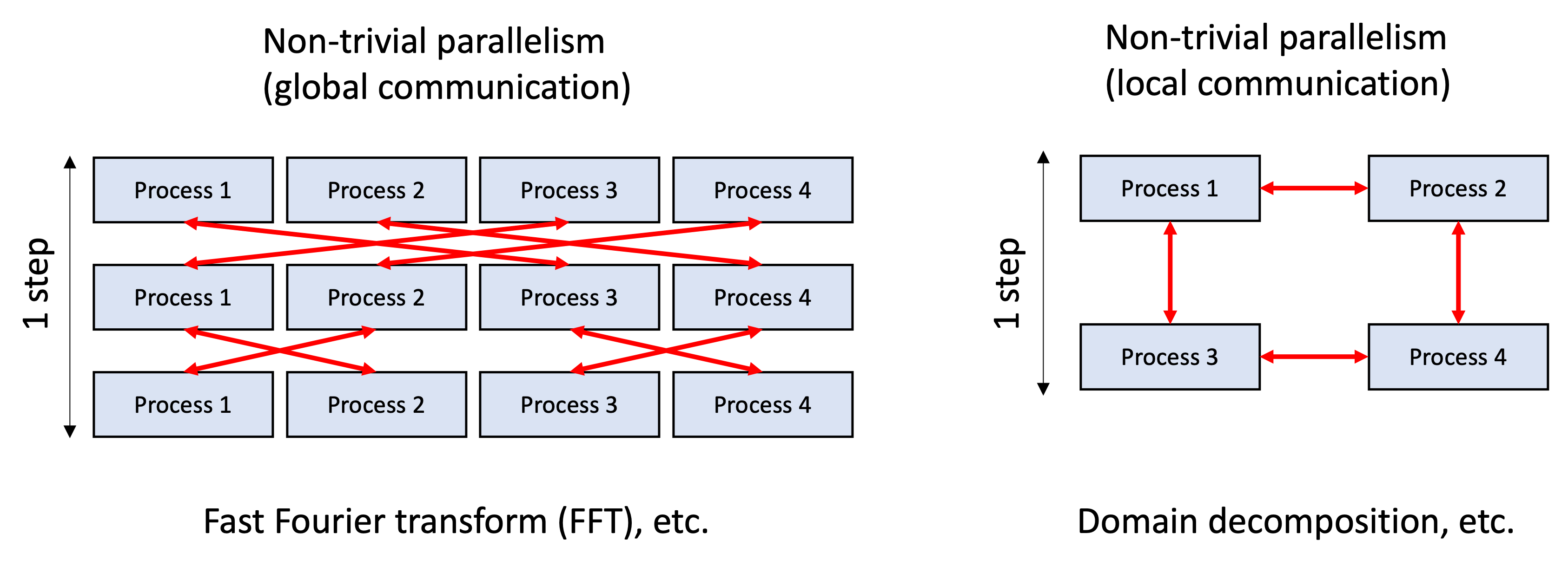
The type requiring all-to-all communication typically appears when a fast Fourier transform is needed. For example, calculating a trillion digits of pi requires multiple-precision arithmetic, which in turn uses Fourier transforms. Fourier transforms are also used in turbulence simulations. A large turbulence simulation once performed on the Earth Simulator would have been difficult without that machine’s powerful network. This kind of all-node communication often uses a butterfly algorithm, but we will not explore it here. Interested readers can search for “parallel FFT.”

Communication only with nearby nodes is typical of domain decomposition. This divides the computational domain among processes, which exchange the information required at adjacent boundaries as they calculate. Process placement matters: logically adjacent regions may be assigned to physically distant nodes, reducing efficiency.

The figure should make all-to-all communication look more demanding. In general, parallelization is easier—and good efficiency easier to achieve—when the volume and frequency of communication are small relative to the amount of computation. The ratio of computation cost to communication cost is sometimes called granularity (we may or may not return to it later).

Here we will use domain decomposition as our example of non-trivial parallelism.

One-Dimensional Diffusion Equation (Serial Version)

As a subject for domain decomposition, consider the one-dimensional diffusion equation. It describes how the temperature of a heated or cooled material changes. If $T(x,t)$ is the temperature at time $t$ and coordinate $x$, and $\kappa$ is the thermal conductivity, then

$$\frac{\partial T}{\partial t} = \kappa \frac{\partial^2 T}{\partial x^2}$$

The steady state is obtained when the time derivative vanishes, so

$$\kappa \frac{\partial^2 T}{\partial x^2} = 0$$

Because the second derivative is zero, we see that the solution is a linear function (or, in related forced cases below, a quadratic function). The solution at an arbitrary time can be obtained with a Fourier transform. Science and engineering students should have encountered this by their second year, so review it if necessary.

To solve this partial differential equation numerically, divide space into $L$ points and discretize it. Use the first-order Euler method in time and a central difference in space. Let the time step be $h$, the spatial interval be 1, and the temperature at site $i$ after step $n$ be $T_i^n$. The temperature at the same site on the next step is

$$T_i^{n+1} = T_i^{n} + h(T_{i+1}^n - 2 T_{i}^n + T_{i-1}^n)$$

If the temperatures at time step $n$ are represented by std::vector<double> lattice, the equation translates directly into code:

  std::copy(lattice.begin(), lattice.end(), orig.begin());
  for (int i = 1; i < L - 1; i++) {
    lattice[i] += h * (orig[i - 1] - 2.0 * orig[i] + orig[i + 1]);
  }

Simple enough. Since this does not update the two endpoints (lattice[0] and lattice[L-1]), impose periodic boundary conditions. Implement the complete update as a function named onestep.

void onestep(std::vector<double> &lattice, const double h) {
  static std::vector<double> orig(L);
  std::copy(lattice.begin(), lattice.end(), orig.begin());
  for (int i = 1; i < L - 1; i++) {
    lattice[i] += h * (orig[i - 1] - 2.0 * orig[i] + orig[i + 1]);
  }
  // For Periodic Boundary
  lattice[0] += h * (orig[L - 1] - 2.0 * lattice[0]  + orig[1]);
  lattice[L - 1] += h * (orig[L - 2] - 2.0 * lattice[L - 1] + orig[0]);
}

That completes the numerical calculation. Let us also write a function that dumps the system state to a file.

void dump(std::vector<double> &data) {
  static int index = 0;
  char filename[256];
  sprintf(filename, "data%03d.dat", index);
  std::cout << filename << std::endl;
  std::ofstream ofs(filename);
  for (int i = 0; i < data.size(); i++) {
    ofs << i << " " << data[i] << std::endl;
  }
  index++;
}

We can now evolve the system in time by supplying suitable conditions. We will try two cases: uniform heating and fixed temperatures. Save the following code as thermal.cpp and run it.

#include <cstdio>
#include <fstream>
#include <iostream>
#include <vector>

const int L = 128;
const int STEP = 100000;
const int DUMP = 1000;

void onestep(std::vector<double> &lattice, const double h) {
  static std::vector<double> orig(L);
  std::copy(lattice.begin(), lattice.end(), orig.begin());
  for (int i = 1; i < L - 1; i++) {
    lattice[i] += h * (orig[i - 1] - 2.0 * orig[i] + orig[i + 1]);
  }
  // For Periodic Boundary
  lattice[0] += h * (orig[L - 1] - 2.0 * lattice[0] + orig[1]);
  lattice[L - 1] += h * (orig[L - 2] - 2.0 * lattice[L - 1] + orig[0]);
}

void dump(std::vector<double> &data) {
  static int index = 0;
  char filename[256];
  sprintf(filename, "data%03d.dat", index);
  std::cout << filename << std::endl;
  std::ofstream ofs(filename);
  for (int i = 0; i < data.size(); i++) {
    ofs << i << " " << data[i] << std::endl;
  }
  index++;
}

void fixed_temperature(std::vector<double> &lattice) {
  const double h = 0.01;
  const double Q = 1.0;
  for (int i = 0; i < STEP; i++) {
    onestep(lattice, h);
    lattice[L / 4] = Q;
    lattice[3 * L / 4] = -Q;
    if ((i % DUMP) == 0) dump(lattice);
  }
}

void uniform_heating(std::vector<double> &lattice) {
  const double h = 0.2;
  const double Q = 1.0;
  for (int i = 0; i < STEP; i++) {
    onestep(lattice, h);
    for (auto &s : lattice) {
      s += Q * h;
    }
    lattice[0] = 0.0;
    lattice[L - 1] = 0.0;
    if ((i % DUMP) == 0) dump(lattice);
  }
}

int main() {
  std::vector<double> lattice(L, 0.0);
  //uniform_heating(lattice);
  fixed_temperature(lattice);
}

The results look like this.

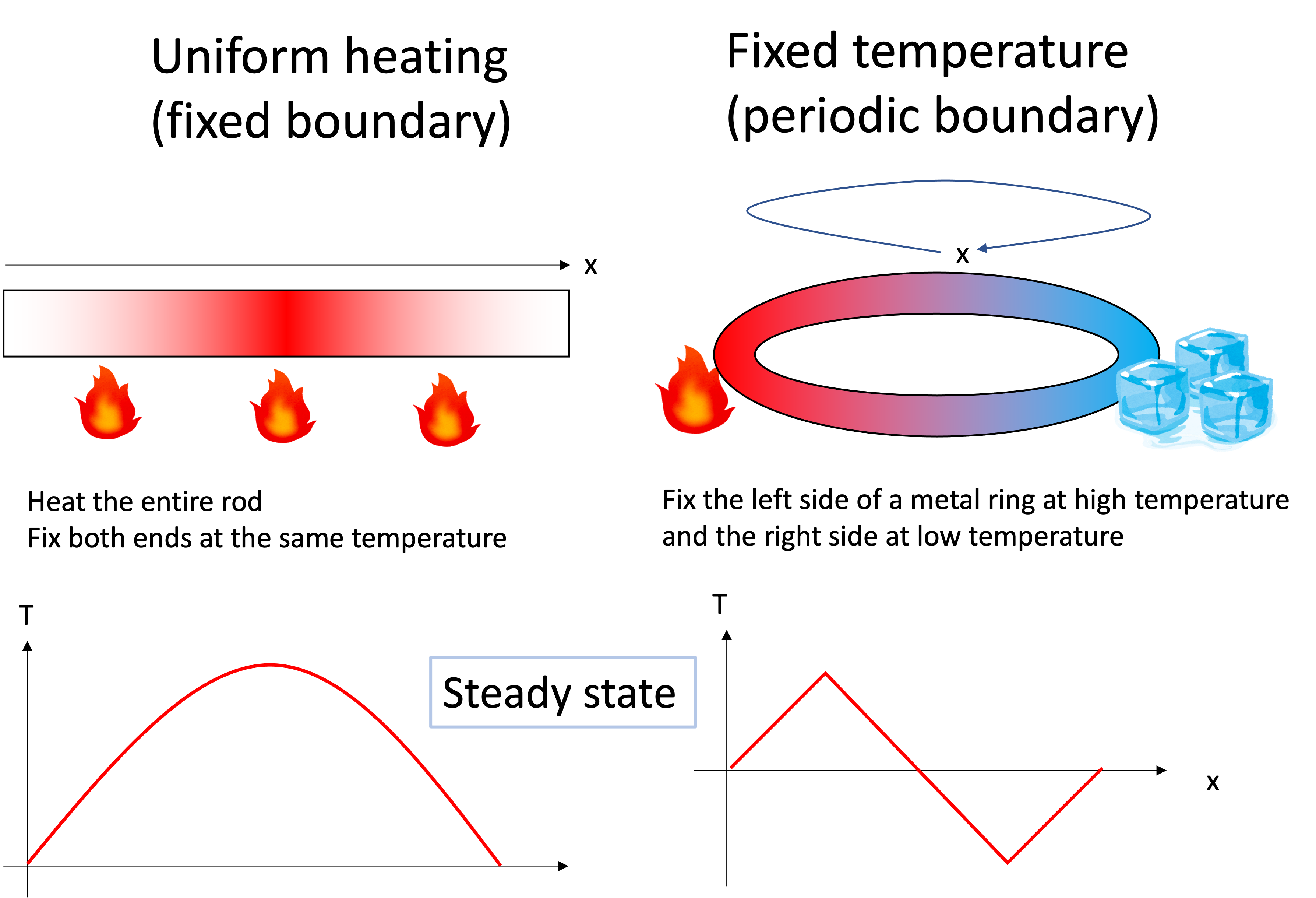
Uniform heating means applying heat evenly throughout the system. If Q is the heat added per unit time, write

    for (auto &s : lattice) {
      s += Q * h;
    }

This alone would make the entire system hotter indefinitely, so fix the temperature at both ends of the rod to zero.

    lattice[0] = 0.0;
    lattice[L - 1] = 0.0;

The calculation can be written as follows.

void uniform_heating(std::vector<double> &lattice) {
  const double h = 0.2;
  const double Q = 1.0;
  for (int i = 0; i < STEP; i++) {
    onestep(lattice, h);
    for (auto &s : lattice) {
      s += Q * h;
    }
    lattice[0] = 0.0;
    lattice[L - 1] = 0.0;
    if ((i % DUMP) == 0) dump(lattice);
  }
}

The system state is written to a file every few steps. The steady state is a quadratic function that vanishes at both ends, specifically

$$T(x) = -x (x-L)$$

Verify that this is quadratic, vanishes at both ends, and solves the heat equation.

The result is shown below.

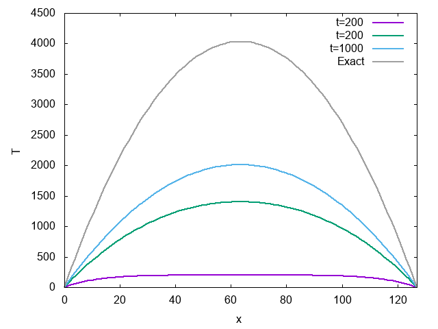
The temperature rises with time and approaches the steady state.

This example does not confirm that the periodic boundary condition works, so let us try fixed temperatures arranged so that heat crosses the boundary. Fix one point on a ring-shaped metal rod at a high temperature and the opposite point at a low temperature. The steady state then consists of straight lines joining the hot and cold points.

The calculation can be written as follows.

void fixed_temperature(std::vector<double> &lattice) {
  const double h = 0.01;
  const double Q = 1.0;
  for (int i = 0; i < STEP; i++) {
    onestep(lattice, h);
    lattice[L / 4] = Q;
    lattice[3 * L / 4] = -Q;
    if ((i % DUMP) == 0) dump(lattice);
  }
}

The result is shown below.

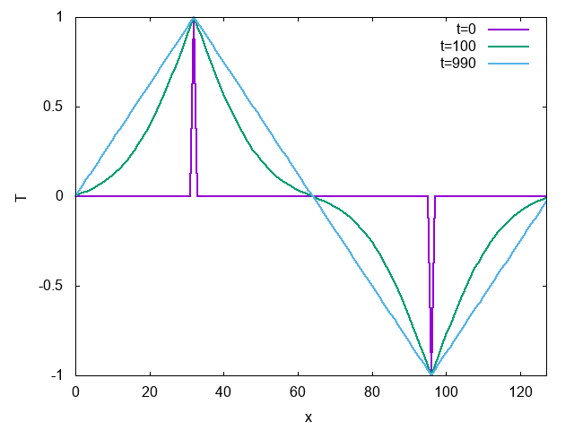
As time passes, the profile approaches the straight-line steady state. The relation governing the temperature gradient in steady-state conduction is known as Fourier’s law—named after the same Fourier as the Fourier transform. Fourier originally developed Fourier series to solve heat-conduction problems.

One-Dimensional Diffusion Equation (Parallel Version)

Now that we have a simulation of the one-dimensional diffusion equation, let us parallelize it with domain decomposition. Divide space among the processes, and let each process update its assigned region while obtaining required information from neighboring processes. Since an update refers to adjacent regions, each process retains a halo, or ghost region, where communicated boundary values are stored.

One issue in parallelization is file output. With a single process, that process simply wrote the file. With process parallelism, however, different processes hold separate pieces of the system state, which must somehow be written out. Before parallelizing the calculation itself, consider how to output data distributed by domain decomposition. Among many possibilities, three straightforward approaches are: every process writes independently, processes append to one file, or the data is gathered before being written.

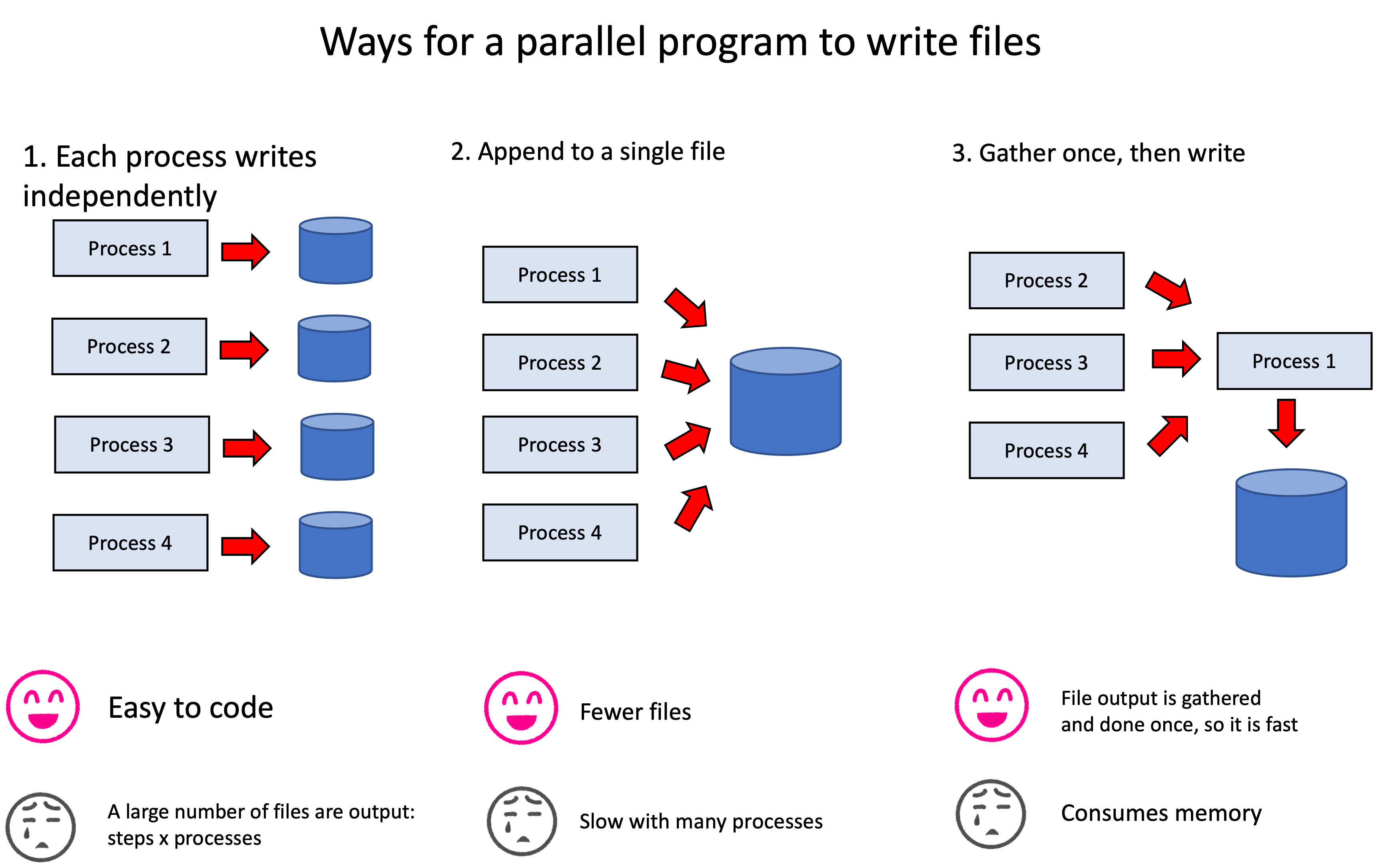
1. Every process writes independently. Each process writes its own file at every output step; process $i$ at step $t$ might write file_t_i.dat. This is easy to code, but creates one file per process per step and therefore an enormous number of files. The files must also be combined for analysis, making management cumbersome.
2. Append to one file. Create one file per step and have the processes append their data sequentially. Analysis is easy because the output matches the serial version, but processes must wait their turn. With several thousand processes, this was painfully slow.
3. Gather, then write. Communicate all data to the root process (rank 0), which writes it in one operation. This performed acceptably with thousands of processes, but gathering every process’s state on one node exhausted memory with tens of thousands.

If memory is not a concern, the third method is convenient, so we will use it here. For memory-intensive calculations or runs with tens of thousands of processes, you will need a more sophisticated approach.

To gather before writing, we must collect data scattered across processes onto one process. MPI provides exactly such a function: MPI_Gather. Its use is easiest to understand from an example. Save the following as gather.cpp and run it.

#include <cstdio>
#include <mpi.h>
#include <vector>

const int L = 8;

int main(int argc, char **argv) {
  MPI_Init(&argc, &argv);
  int rank, procs;
  MPI_Comm_rank(MPI_COMM_WORLD, &rank);
  MPI_Comm_size(MPI_COMM_WORLD, &procs);
  const int mysize = L / procs;
  // Local data (initialized with this process's rank)
  std::vector<int> local(mysize, rank);
  // Global buffer that receives the gathered data
  std::vector<int> global(L);
  // Communication (gather on rank 0)
  MPI_Gather(local.data(), mysize, MPI_INT, global.data(), mysize, MPI_INT, 0,  MPI_COMM_WORLD);

  // Rank 0 prints the result
  if (rank == 0) {
    for (int i = 0; i < L; i++) {
      printf("%d", global[i]);
    }
    printf("\n");
  }
  MPI_Finalize();
}

This models a length-L=8 data set divided so that every process holds mysize = L/procs elements. Each process stores its portion in local, initialized with its own rank. The program gathers everything onto rank 0, receives it in global, and prints it.

The output is as follows.

$ mpic++ gather.cpp
$ mpirun -np 1 ./a.out
00000000

$ mpirun -np 2 ./a.out
00001111

$ mpirun -np 4 ./a.out
00112233

$ mpirun -np 8 ./a.out
01234567

We tried divisions from one through eight processes. Once this works, parallelizing the one-dimensional heat equation is not difficult. After gathering all data, pass it to the serial dump routine with a function like this.

void dump_mpi(std::vector<double> &local, int rank, int procs) {
  static std::vector<double> global(L);
  MPI_Gather(&(local[1]), L / procs, MPI_DOUBLE, global.data(), L / procs, MPI_DOUBLE, 0,  MPI_COMM_WORLD);
  if (rank == 0) {
    dump(global);
  }
}

Each process stores its data in a std::vector named local. Because it has a halo at each end, MPI_Gather excludes those entries and collects the interior into the std::vector named global. Rank 0 then calls the serial dump function dump.

With output settled, let us parallelize the calculation. Because this is a finite-difference equation, provide a one-site halo at each end and communicate only those sites with neighboring processes.

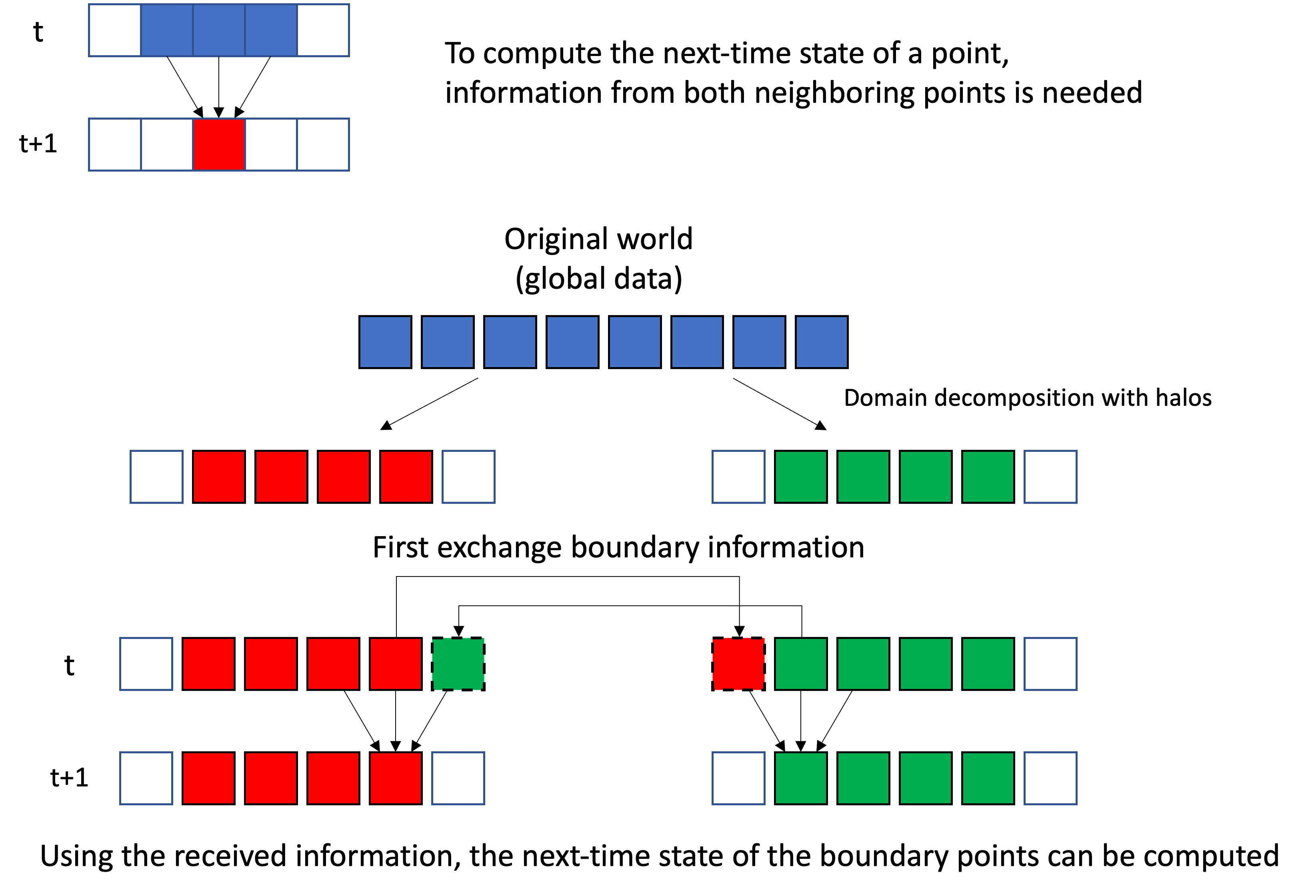
Before each update, copy boundary values from the processes responsible for the regions on either side into the halos, then perform the calculation normally. This uses point-to-point communication. MPI provides MPI_Send and MPI_Recv as its basic send and receive operations, but MPI_Sendrecv, which performs both together, is preferable to pairing them manually. Separate sends and receives can deadlock, and MPI_Sendrecv generally performs better. The parallel update is therefore as follows.

void onestep(std::vector<double> &lattice, double h, int rank, int procs) {
  const int size = lattice.size();
  static std::vector<double> orig(size);
  std::copy(lattice.begin(), lattice.end(), orig.begin());
  // Communication begins here
  const int left = (rank - 1 + procs) % procs; // Rank to the left
  const int right = (rank + 1) % procs; // Rank to the right
  MPI_Status st;
  // Send the right edge rightward and receive the left edge from the left
  MPI_Sendrecv(&(lattice[size - 2]), 1, MPI_DOUBLE, right, 0, &(orig[0]), 1, MPI_DOUBLE, left, 0, MPI_COMM_WORLD, &st);
  // Send the left edge leftward and receive the right edge from the right
  MPI_Sendrecv(&(lattice[1]), 1, MPI_DOUBLE, left, 0, &(orig[size - 1]), 1, MPI_DOUBLE, right, 0, MPI_COMM_WORLD, &st);

  // The rest is identical to the serial version
  for (int i = 1; i < size - 1; i++) {
    lattice[i] += h * (orig[i - 1] - 2.0 * orig[i] + orig[i + 1]);
  }
}

The comments describe everything, and there is nothing especially difficult here. Note that in MPI_Sendrecv, the destination process differs from the source process. Imagine everyone standing in a circle at a holiday gift exchange, handing a gift to the person on the right and receiving one from the person on the left. Sending right and receiving from the right would also work, but sending right and receiving from the left makes the code simpler and, in the author’s experience, faster.

With the update complete, we can add physical conditions to create the simulation. First, uniform heating:

void uniform_heating(std::vector<double> &lattice, int rank, int procs) {
  const double h = 0.2;
  const double Q = 1.0;
  for (int i = 0; i < STEP; i++) {
    onestep(lattice, h, rank, procs);
    for (auto &s : lattice) {
      s += Q * h;
    }
    if (rank == 0) {
      lattice[1] = 0.0;
    }
    if (rank == procs - 1) {
      lattice[lattice.size() - 2] = 0.0;
    }
    if ((i % DUMP) == 0) dump_mpi(lattice, rank, procs);
  }
}

This is almost identical to the serial version. When fixing the temperatures at both ends, however, rank 0 owns the left endpoint and rank procs-1 owns the right, so these assignments require conditionals. The only other change is replacing dump with dump_mpi.

Next, the fixed-temperature condition:

void fixed_temperature(std::vector<double> &lattice, int rank, int procs) {
  const double h = 0.01;
  const double Q = 1.0;
  const int s = L / procs;
  for (int i = 0; i < STEP; i++) {
    onestep(lattice, h, rank, procs);
    if (rank == (L / 4 / s)) {
      lattice[L / 4 - rank * s + 1] = Q;
    }
    if (rank == (3 * L / 4 / s)) {
      lattice[3 * L / 4 - rank * s + 1] = -Q;
    }
    if ((i % DUMP) == 0) dump_mpi(lattice, rank, procs);
  }
}

As with uniform heating, we must determine which local position on which process owns each fixed-temperature point, but this is not especially difficult. Save the completed parallel program as thermal_mpi.cpp.

#include <cstdio>
#include <fstream>
#include <iostream>
#include <mpi.h>
#include <vector>

const int L = 128;
const int STEP = 100000;
const int DUMP = 1000;

void dump(std::vector<double> &data) {
  static int index = 0;
  char filename[256];
  sprintf(filename, "data%03d.dat", index);
  std::cout << filename << std::endl;
  std::ofstream ofs(filename);
  for (unsigned int i = 0; i < data.size(); i++) {
    ofs << i << " " << data[i] << std::endl;
  }
  index++;
}

void dump_mpi(std::vector<double> &local, int rank, int procs) {
  static std::vector<double> global(L);
  MPI_Gather(&(local[1]), L / procs, MPI_DOUBLE, global.data(), L / procs, MPI_DOUBLE, 0, MPI_COMM_WORLD);
  if (rank == 0) {
    dump(global);
  }
}

void onestep(std::vector<double> &lattice, double h, int rank, int procs) {
  const int size = lattice.size();
  static std::vector<double> orig(size);
  std::copy(lattice.begin(), lattice.end(), orig.begin());
  // Communication begins here
  const int left = (rank - 1 + procs) % procs; // Rank to the left
  const int right = (rank + 1) % procs;        // Rank to the right
  MPI_Status st;
  // Send the right edge rightward and receive the left edge from the left
  MPI_Sendrecv(&(lattice[size - 2]), 1, MPI_DOUBLE, right, 0, &(orig[0]), 1, MPI_DOUBLE, left, 0, MPI_COMM_WORLD, &st);
  // Send the left edge leftward and receive the right edge from the right
  MPI_Sendrecv(&(lattice[1]), 1, MPI_DOUBLE, left, 0, &(orig[size - 1]), 1, MPI_DOUBLE, right, 0, MPI_COMM_WORLD, &st);

  // The rest is identical to the serial version
  for (int i = 1; i < size - 1; i++) {
    lattice[i] += h * (orig[i - 1] - 2.0 * orig[i] + orig[i + 1]);
  }
}

void uniform_heating(std::vector<double> &lattice, int rank, int procs) {
  const double h = 0.2;
  const double Q = 1.0;
  for (int i = 0; i < STEP; i++) {
    onestep(lattice, h, rank, procs);
    for (auto &s : lattice) {
      s += Q * h;
    }
    if (rank == 0) {
      lattice[1] = 0.0;
    }
    if (rank == procs - 1) {
      lattice[lattice.size() - 2] = 0.0;
    }
    if ((i % DUMP) == 0) dump_mpi(lattice, rank, procs);
  }
}

void fixed_temperature(std::vector<double> &lattice, int rank, int procs) {
  const double h = 0.01;
  const double Q = 1.0;
  const int s = L / procs;
  for (int i = 0; i < STEP; i++) {
    onestep(lattice, h, rank, procs);
    if (rank == (L / 4 / s)) {
      lattice[L / 4 - rank * s + 1] = Q;
    }
    if (rank == (3 * L / 4 / s)) {
      lattice[3 * L / 4 - rank * s + 1] = -Q;
    }
    if ((i % DUMP) == 0) dump_mpi(lattice, rank, procs);
  }
}

int main(int argc, char **argv) {
  MPI_Init(&argc, &argv);
  int rank, procs;
  MPI_Comm_rank(MPI_COMM_WORLD, &rank);
  MPI_Comm_size(MPI_COMM_WORLD, &procs);
  const int mysize = L / procs + 2;
  std::vector<double> local(mysize);
  uniform_heating(local, rank, procs);
  //fixed_temperature(local, rank, procs);
  MPI_Finalize();
}

Now that the program is parallel, let us see whether it became faster by running the uniform-heating case.

First, the serial version:

$ clang++ -O3 -std=c++11 thermal.cpp
$ time ./a.out
data000.dat
data001.dat
(snip)
data099.dat
./a.out  0.05s user 0.12s system 94% cpu 0.187 total

Next, the parallel version:

$ time mpirun -np 2 --oversubscribe ./a.out
data000.dat
data001.dat
(snip)
data099.dat
mpirun -np 2 --oversubscribe ./a.out  0.42s user 0.16s system 176% cpu 0.330 total

$ time mpirun -np 4 --oversubscribe ./a.out
data000.dat
data001.dat
(snip)
data099.dat
mpirun -np 4 --oversubscribe ./a.out  1.73s user 0.88s system 234% cpu 1.116 total

$ time mpirun -np 8 --oversubscribe ./a.out
data000.dat
data001.dat
(snip)
data099.dat
mpirun -np 8 --oversubscribe ./a.out  3.28s user 2.89s system 311% cpu 1.980 total

Indeed, increasing the process count successfully made it slower.

Hooray!

The system is small and one-dimensional, so the computation is extremely light; the extra work required for communication was predictably more expensive than the computation it replaced. Nevertheless, this code contains all the fundamental techniques of domain decomposition. Once you understand it, you can in principle parallelize any explicit finite-difference code, so the technique has broad applications.

Aside: Eager and Rendezvous Protocols

Earlier, we said that using MPI_Send and MPI_Recv can cause deadlock. Suppose process 0 sends to and receives from process 1, while process 1 likewise sends to and receives from process 0. Process 0 cannot proceed until its send receives a response from process 1. But process 1 also cannot proceed until its send receives a response from process 0, and neither reaches the receive that would satisfy the other’s send. This appears certain to deadlock, yet in practice it often does not when the messages are small.

The reason is that small messages use the eager protocol, while larger messages use the rendezvous protocol. In the rendezvous protocol, the sender first asks, “May I send this much data?” The receiver confirms that it can provide a buffer and replies, “Yes.” Data transfer begins only after this handshake. Because each side must await the other’s response, deadlock is possible. Moreover, if the receiver is already known to have buffer space, making the sender wait for confirmation wastes time.

The eager protocol instead assumes that the receiver always has a buffer of some predetermined size, and the sender deposits the data there immediately. It resembles a delivery service leaving a small parcel in a mailbox or designated location rather than arranging redelivery. The receiver copies the data from that buffer when convenient. Since the sender completes MPI_Send and continues without waiting for a response, the preceding example does not deadlock.

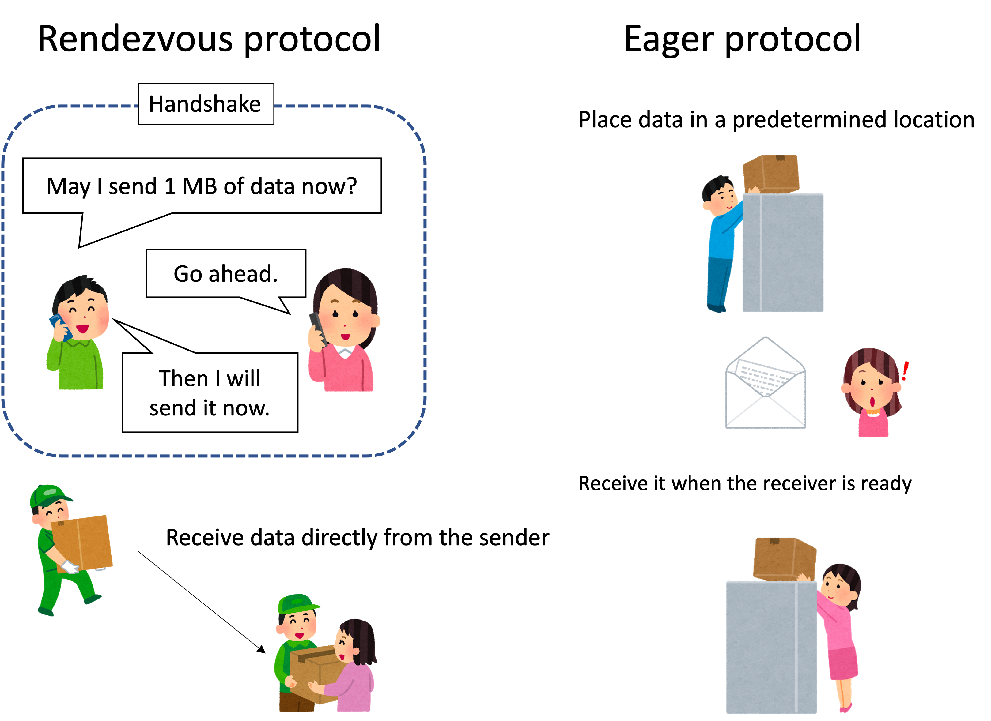
MPI switches between eager and rendezvous protocols according to message size, and the threshold varies by system. Code with a potential MPI_Send/MPI_Recv deadlock may therefore work at one site but deadlock at another, or work for a small system but deadlock when the system grows, creating an especially confusing bug. MPI_Sendrecv avoids this problem, so prefer it whenever possible.

Because MPI_Send and MPI_Recv are called blocking communication, they are sometimes misunderstood to mean that execution never proceeds until the peer responds. As the eager protocol shows, execution may continue regardless of a response. Blocking communication guarantees that when MPI_Recv completes, the receive buffer contains the data. With nonblocking communication, the result is not guaranteed until MPI_Wait, which completes the operation, has returned. For further detail, see the following lecture notes.

Fundamentals of Parallel Programming (Atsushi Hori, in Japanese)