Day 6: Hybrid Parallelism
So far, we have used MPI for “process parallelism” as our means of parallelization. As mentioned at the beginning, another means of parallelization is “thread parallelism.” Process parallelism uses a distributed-memory model, while thread parallelism uses a shared-memory model. Since thread parallelism alone cannot span nodes, process parallelism is normally essential when we talk about “using a supercomputer.” Parallelization using only MPI-based process parallelism is called “flat MPI.” In contrast, parallelization that combines process parallelism and thread parallelism is called “hybrid parallelism.” Naturally, hybrid parallelism is more troublesome than either process parallelism or thread parallelism alone, so we would rather avoid it if possible. Depending on the application and problem size, however, there may be cases where hybrid parallelism is the only practical choice. Here, we will look at points to keep in mind when using thread parallelism and at a real example of hybrid parallelism.
Virtual Memory and the TLB
Section titled “Virtual Memory and the TLB”One issue that did not require much attention with process parallelism, but does with thread parallelism, is NUMA. To understand NUMA, you first need to know about virtual memory. So let us take a look at virtual memory.
An OS does many different things, but one particularly important job is memory management. Physically, “memory” refers to the DRAM installed on the motherboard, but the “memory” visible to a process running under the OS is a virtualized version of it. Memory that appears contiguous to a process may in fact be scattered across DRAM. The OS neatly translates between “addresses visible to the process” and “addresses physically allocated in DRAM,” so the process does not have to be aware of physical memory. This mechanism is called virtual memory. The advantages of virtual memory include:
- Because the OS manages memory, multiple processes do not need to worry about one another’s memory (which is also desirable for security)
- Memory that is physically noncontiguous can appear as contiguous addresses to a process
- When memory is insufficient, swapping to a hard disk or other storage provides a logical address space larger than physical memory
Note that Windows appears to use the term “virtual memory” for the upper limit of the area swapped to disk, so be careful about the distinction.
Let us see that each process is actually given its own virtual memory. Write the following code (vmem.cpp).
#include <cstdio>#include <mpi.h>
int rank;
int main(int argc, char **argv) {  MPI_Init(&argc, &argv);  MPI_Comm_rank(MPI_COMM_WORLD, &rank);  printf("rank = %d, address = %x\n", rank, &rank);  MPI_Finalize();}
This code prints the value and address of the int variable rank.
Putting it inside a function would give it an address on the stack (which would actually be fine too),
so it is declared as a global variable. Running this on Linux produces something like the following.
$ mpic++ vmem.cpp$ mpirun -np 4 ./a.outrank = 0, address = 611e64rank = 1, address = 611e64rank = 3, address = 611e64rank = 2, address = 611e64You can see that the values differ even though all the addresses are the same. This is because the address spaces “visible” from each of the four launched processes are physically mapped to different addresses.
Running the code above on a Mac instead produces this.
$ mpirun -np 4 --oversubscribe ./a.outrank = 1, address = cae26d8rank = 2, address = fe426d8rank = 3, address = ff4c6d8rank = 0, address = 40c36d8You can see that rank, which should logically be in the same location, has completely different addresses.
This is because macOS employs a security technique called Address Space Layout Randomization (ASLR).
Some Linux distributions may do this as well. But let us set that aside.
This is a slight digression from the main topic, but since virtual memory has come up, let us also discuss the TLB.
The OS manages the “logical addresses” visible to a process and the “physical addresses” actually allocated in DRAM
in units called pages. Memory is divided into chunks of a certain size, each called a page.
The mapping between logical and physical addresses is called a page table entry (PTE), and the collection of these entries is called a page table.
When a process requests a memory access, the page table must be consulted to translate the process’s logical address into a physical address.
Use getconf to check the page size.
$ getconf PAGESIZE4096Page sizes are commonly set to 4096 bytes. This means that 1 GB of memory is managed by 262,144 PTEs. It is impossible to fit this many entries in cache, so page tables are basically stored in memory. Consequently, when a cache miss occurs during a memory access, memory must first be accessed to translate the logical address into a physical address, and then, once the physical address is known, that address must be accessed: two memory accesses in total. To prevent this, a special cache stores PTEs that have already been accessed. This is the TLB (Translation Lookaside Buffer). Since it is also a kind of cache, it has a hierarchy such as L1 and L2, just like an ordinary cache. Cache size is specified in bytes, whereas TLB size is specified by the number of entries. x86info is useful for viewing TLB information.
On CentOS, install it with:
sudo yum install x86infoIt is probably included in the package repositories of most other distributions as well. Specify -c to view cache information.
The following result was obtained on an Intel Xeon Gold 6130 (Skylake).
x86info v1.31preFound 32 identical CPUsExtended Family: 0 Extended Model: 5 Family: 6 Model: 85 Stepping: 4Type: 0 (Original OEM)CPU Model (x86info's best guess): Core i7 (Skylake-X)Processor name string (BIOS programmed): Intel(R) Xeon(R) Gold 6130 CPU @ 2.10GHz
Cache info L1 Data Cache: 32KB, 8-way associative, 64 byte line size L1 Instruction Cache: 32KB, 8-way associative, 64 byte line size L2 Unified Cache: 1024KB, 16-way associative, 64 byte line size L3 Unified Cache: 22528KB, 11-way associative, 64 byte line sizeTLB info Instruction TLB: 2M/4M pages, fully associative, 8 entries Instruction TLB: 4K pages, 8-way associative, 128 entries Data TLB: 1GB pages, 4-way set associative, 4 entries Data TLB: 4KB pages, 4-way associative, 64 entries Shared L2 TLB: 4KB/2MB pages, 6-way associative, 1536 entries 64 byte prefetching.Total processor threads: 32This system has 2 eight-core processors with hyper-threading (2 threads per core) running at an estimated 2.10GHz
Anyone familiar with cache organization will recognize a cache-like structure: separate instruction and data TLBs, distinct L1 and L2 levels, and a shared L2 for instructions and data. Yet even the largest TLB has only 1,536 entries. With the default 4 KB pages, fully utilizing it can manage only a little over 6 MB of address space. Handling more data than that will therefore cause TLB misses.
However, as the preceding output says, Shared L2 TLB: 4KB/2MB pages, so this TLB can also manage 2 MB pages. If each page is 2 MB, 1,536 entries can cover 3 GB of address space. Using pages larger than the ordinary size in this way is called using large pages or huge pages. The large-page size can be checked in meminfo.
$ cat /proc/meminfo |grep HugepagesizeHugepagesize: 2048 kBThis confirms that it is indeed 2 MB. Large pages can be expected to reduce TLB misses, but because the minimum unit of memory management becomes larger, more memory is wasted and effective memory usage increases. It is also worth remembering that large pages are not swapped out. With virtual memory, when memory runs short, pages are swapped to disk, but large pages are not swapped. If a large page were swapped out (written to disk), then when it later became necessary and had to be swapped in (read back into memory), a contiguous region of physical memory the size of that large page would have to be provided. Fragmentation and similar issues mean that this cannot be guaranteed.
Aside: TLB Misses
Section titled “Aside: TLB Misses”The TLB is also a type of cache, so just like an ordinary cache, it can suffer from cache misses. When a TLB miss occurs, the CPU must walk through the page tables to find the physical address corresponding to a virtual address.
If all 64 bits of an address were used, it would theoretically be possible to represent a virtual address space of bytes, or 16 EiB. In practice, however, x86-64 does not use all 64 bits for address translation. Here, let us consider a typical four-level paging scheme that uses the lower 48 bits.
These 48 bits are divided into five parts. The lowest 12 bits form an offset specifying a location within a page. Since 12 bits can represent bytes, the standard page size is 4 KiB. The remaining 36 bits are divided into four groups of 9 bits, each of which is used to traverse one level of the page-table hierarchy. As an analogy, we can think of these four 9-bit fields as levels of a U.S. address, such as “California,” “San Francisco,” “Market Street,” and “1355.” The final 12 bits then correspond to a room number within the building.
Given a virtual address, the CPU first uses the highest 9 bits to look up an entry in the first address book. That entry tells the CPU where the next address book is located in physical memory. It then uses the next 9 bits to look up an entry in that address book and proceeds to the next one. After repeating this process through four levels, the CPU finally determines the location of the target physical page. This process of traversing page tables to translate a virtual address into a physical address is called a page walk.
When a 2 MiB large page is used, on the other hand, the 9 bits that would normally be used to select an entry in the last-level page table are instead used as part of the offset within the page. The offset therefore consists of 12+9=21 bits, giving a page size of bytes, or 2 MiB. In terms of the address analogy, this is like removing one level from the address hierarchy and replacing the final building with an enormous skyscraper. Because a large page allows a single TLB entry to cover a much larger region of memory, it can reduce the number of TLB misses for a TLB of the same size.
In any case, page walks take time, so it is natural to want to cache page table entries once they have been looked up. That is what the TLB does. The CPU contains a hardware TLB just as it contains hardware caches. In general, TLB misses are expensive because they involve a page walk. However, frequent TLB misses mean that the program is touching far more pages than the TLB has entries. That implies poor locality in memory usage, so cache misses are also likely to be occurring. Frequent cache misses completely destroy performance, so ordinarily those are more often the main problem, and fixing them will often reduce TLB misses at the same time (or so it seems). In practice, though, there are occasional cases where cache misses are not much of a problem but TLB misses have a serious impact.
This is a fairly advanced topic, but caches store data using a hash-like mechanism. Roughly speaking, a hash value is created from a logical address, and that hash determines where in the cache the memory is placed. As a result, data from different locations in memory can end up in the same cache location because their hash values collide. If a program is unlucky enough to access those items alternately, it repeatedly brings the same data into and evicts it from the cache even though the cache has plenty of total capacity, causing extreme performance degradation. This is called cache thrashing. If you are working with a multidimensional array and performance degrades dramatically only at one particular size when a dimension is changed, cache thrashing is a likely cause.
Since the TLB is also a cache, thrashing occurs there by exactly the same principle. This is called TLB thrashing. In my own experience, at one site my code performed perfectly well at high parallelism with flat MPI, but when changed to hybrid parallelism, its performance fluctuated at high parallelism despite performing a completely equivalent computation, resulting in substantial degradation. While removing unnecessary routines to hunt for the culprit, I eventually found this situation: linking an object file containing a function that was never called degraded performance, while omitting it did not. To repeat, performance varied by nearly 20% depending on whether an object file containing an unused function was linked. This did not happen with flat MPI; it happened only with hybrid parallelism. It ultimately turned out to be TLB thrashing, and changing the page size suppressed the performance degradation. Even now, however, I do not really understand why hybrid parallelism caused the TLB thrashing. Kazushige Goto, famous for GotoBLAS, has also pointed out in several papers that the TLB has a major impact on matrix multiplication.
- On Reducing TLB Misses in Matrix Multiplication (2002) by Kazushige Goto and Robert van de Geijn
- Anatomy of high-performance matrix multiplication
Apparently, there are also quite a few cases where performance fluctuates during hybrid execution and consequently degrades parallel performance, with TLB misses suspected as the cause. The details seem to depend heavily on implementation: how the hardware handles the TLB, and what it does under multithreading versus multiprocessing. My honest feeling as the author is that I do not really know what is going on there.
As an aside to this aside, logical addresses are 8-byte aligned, so the lowest three bits are always zero when an address is written in binary. glibc’s malloc uses these bits to record the state of memory (chunks). For details, see kosaki’s malloc video or Journey through malloc (glibc edition).
A compute node consists of “memory” and “CPUs,” but CPUs have recently become multicore and multisocket, making the internals of a node quite complex.
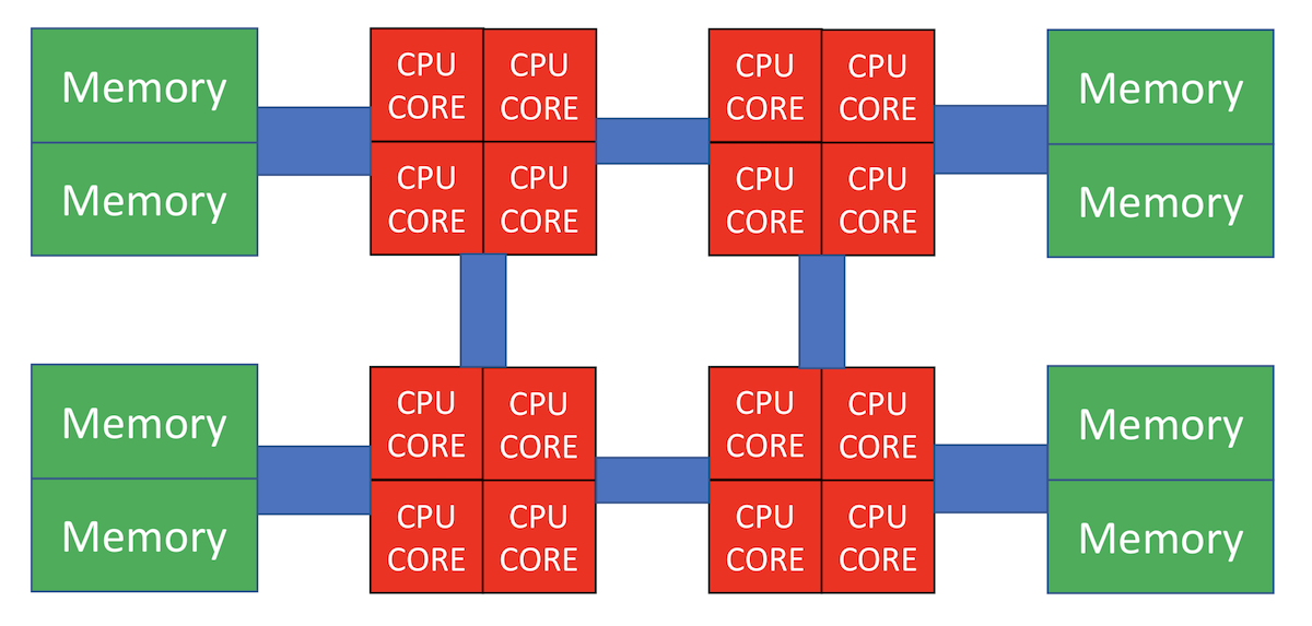
In the figure above, four CPUs are installed, each connected to memory. The CPUs are also connected to one another by a bus, so, for example, the CPU at the lower left can access the memory at the upper right. Doing so, however, takes longer than accessing memory connected nearby. A configuration in which memory can be “near” or “far” from a CPU in this way is called Non-uniform Memory Access (NUMA). I do not know how NUMA is usually pronounced, but I pronounce it “noo-ma.” Some people also pronounce it “numa” or “new-ma.” We will not go deeply into why NUMA is needed here; interested readers should investigate it themselves.
Simply declaring logical memory does not yet allocate physical memory. For example, suppose we have the following array declaration.
double a[4096];Because one double-precision floating-point number occupies 8 bytes, if the page size is 4,096 bytes, eight pages must be allocated for this entire array. Physical memory is not allocated at the instant of declaration, however. It is allocated the first time the array is accessed. When the array is first touched, its corresponding page is allocated in physical memory, and the chosen memory is the memory nearest to the core on which the thread that touched it was running. This is called the first-touch policy. Once physical memory has been allocated, it remains there until it is released. Consequently, access from a thread running on a distant core will take longer.
With flat MPI, each process has its own independent logical memory, so in principle a page touched by one process’s main thread will not later be touched by another thread (we are not considering process migration or similar behavior here). With thread parallelism, however, the thread that first touches a page may differ from the thread that performs the computation.
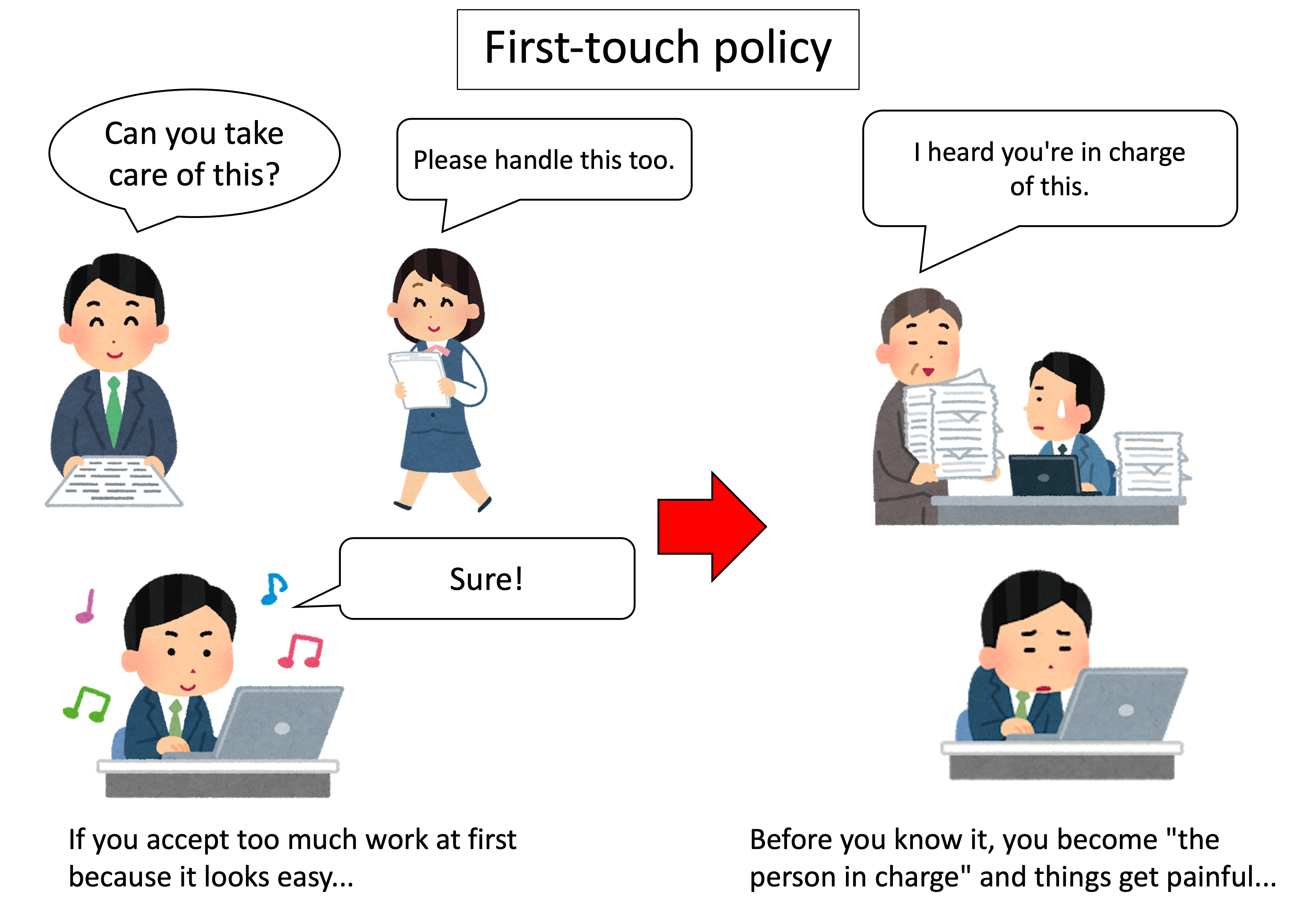
This becomes a problem when, reasoning that “initialization is cheap,” a large array is initialized by the main thread. All its pages are then allocated near the main thread, and when the heavy computation begins, every thread sends data requests to the CPU running the main thread, slowing everything down. To prevent this, the threads that will process the pages later must be made to touch those pages first.
OpenMP Example
Section titled “OpenMP Example”We will now finally use OpenMP for thread parallelism, but first let us profile the serial code.
Profiling means analyzing the performance of executable code; at its simplest, it determines which functions consume how much time.
perf is a good tool for performance analysis. Unfortunately, macOS has no equivalent to perf, and gprof, which is used for similar purposes, does not work properly either.
The following discussion therefore assumes Linux, where perf is available. The execution environment is as follows.
- Intel(R) Xeon(R) CPU E5-2680 v3 @ 2.50GHz, 12 cores x 2 sockets
For our serial code, let us use the Gray-Scott model computation from Day 4. gs.cpp removes intermediate file output so that only the computation itself is counted, and also measures the execution time.
https://github.com/kaityo256/sevendayshpc/blob/main/examples/day6/gs.cpp
For debugging, however, it does write the final result to a file. Let us compile it and profile it with perf. First, record a profile with perf record.
$ g++ -O3 -mavx2 -std=c++11 -fopenmp gs.cpp -o gs.out$ perf record ./gs.out2527 [ms]conf000.dat[ perf record: Woken up 1 times to write data ][ perf record: Captured and wrote 0.113 MB perf.data (~4953 samples) ]We can see that the execution time was 2,527 ms and that conf000.dat was written. For later use, rename it to something like conf000.org.
The profile data recorded by perf is saved as perf.data. Its contents can be viewed with perf report.
perf reportDepending on the environment, a screen like this will appear.
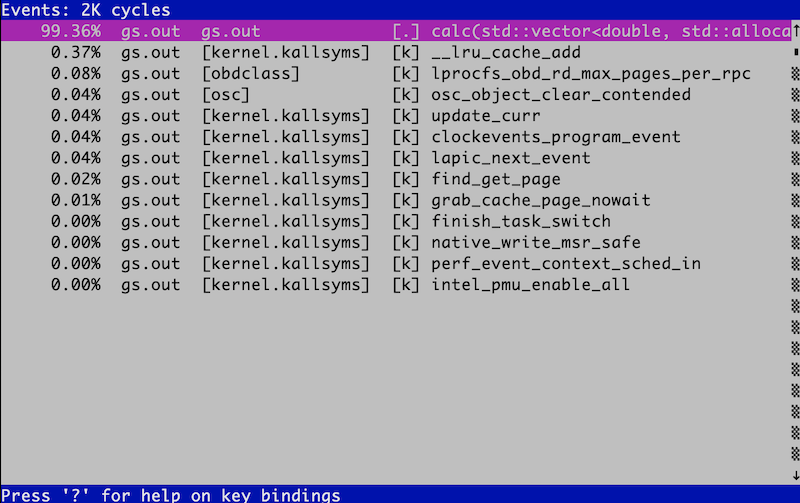
It displays various things, but for now it is enough to confirm that the main computation routine, calc, accounts for 99.36% of the computation time.
The “heaviest” function is called the hotspot. Computational code in which the hotspot accounts for at least 90% is easy to tune.
The heaviest function looks like this.
void calc(vd &u, vd &v, vd &u2, vd &v2) {// Outer loop for (int iy = 1; iy < L - 1; iy++) { // Inner loop for (int ix = 1; ix < L - 1; ix++) { double du = 0; double dv = 0; const int i = ix + iy * L; du = Du * laplacian(ix, iy, u); dv = Dv * laplacian(ix, iy, v); du += calcU(u[i], v[i]); dv += calcV(u[i], v[i]); u2[i] = u[i] + du * dt; v2[i] = v[i] + dv * dt; } }}This is a nested loop. OpenMP parallelizes a loop by inserting a directive immediately before it to instruct the compiler, “Parallelize this loop.” When using thread parallelism, we must check whether dependencies exist between loop indices. Here, there happen to be no dependencies at all between loop indices, so we may parallelize it however we like (rather than pure coincidence, of course, the example was chosen to have this property).
First, let us put a directive on the inner loop. We need only insert the #pragma omp parallel for directive immediately before the target loop.
https://github.com/kaityo256/sevendayshpc/blob/main/examples/day6/gs_omp1.cpp
void calc(vd &u, vd &v, vd &u2, vd &v2) { for (int iy = 1; iy < L - 1; iy++) {#pragma omp parallel for for (int ix = 1; ix < L - 1; ix++) { double du = 0; double dv = 0; const int i = ix + iy * L; du = Du * laplacian(ix, iy, u); dv = Dv * laplacian(ix, iy, v); du += calcU(u[i], v[i]); dv += calcV(u[i], v[i]); u2[i] = u[i] + du * dt; v2[i] = v[i] + dv * dt; } }}Let us run it. The number of threads is specified with the OMP_NUM_THREADS environment variable. This is a 12-core, 2-socket machine, so it has 24 cores in total; let us run with 24 threads. We will also use the time command to see how much of the CPU is being used.
$ time OMP_NUM_THREADS=24 ./gs_omp1.out24 threads 24078 [ms]conf000.datOMP_NUM_THREADS=24 ./gs_omp1.out 573.12s user 1.72s system 2384% cpu 24.103 totalThe 2,384% figure indicates that all 24 cores are indeed being used, but code that took 2,527 ms in serial now takes 24,078 ms. In other words, parallelization made it ten times slower. While we are at it, let us also confirm that the result is correct (fundamental!).
diff conf000.org conf000.datIt looks fine.
Next, let us parallelize the outer loop.
https://github.com/kaityo256/sevendayshpc/blob/main/examples/day6/gs_omp2.cpp
void calc(vd &u, vd &v, vd &u2, vd &v2) {#pragma omp parallel for for (int iy = 1; iy < L - 1; iy++) { for (int ix = 1; ix < L - 1; ix++) { double du = 0; double dv = 0; const int i = ix + iy * L; du = Du * laplacian(ix, iy, u); dv = Dv * laplacian(ix, iy, v); du += calcU(u[i], v[i]); dv += calcV(u[i], v[i]); u2[i] = u[i] + du * dt; v2[i] = v[i] + dv * dt; } }}Let us perform the same computation.
$ time OMP_NUM_THREADS=24 ./gs_omp2.out24 threads 411 [ms]conf000.datOMP_NUM_THREADS=24 ./gs_omp2.out  9.16s user 0.02s system 2194% cpu 0.418 total
$ diff conf000.org conf000.dat
This time it became faster. The result also appears correct. Nevertheless, despite using 24 cores, it is only 6.4 times faster, for a parallel efficiency of about 27%. Incidentally, changing the run to 12 threads makes little difference to the execution time.
$ time OMP_NUM_THREADS=12 ./gs_omp2.out12 threads 410 [ms]conf000.datOMP_NUM_THREADS=12 ./gs_omp2.out 4.91s user 0.01s system 1185% cpu 0.415 totalBecause halving the degree of parallelism barely changes the execution time, the parallel efficiency improves to 51%. This demonstrates that:
- Performance changes completely depending on whether the inner or outer loop of a nested loop is parallelized. Parallelization can even make the code slower.
- Increasing the number of threads does not necessarily improve performance. Beyond some point, adding threads may instead degrade it.
Now let us see why parallelization made the code slower. First, here is a profile of the code with the directive on the inner loop, run with one thread.
To make it easier to read, pipe the output of perf report to cat. By default, perf report displays results through a TUI interface (--tui),
but when connected to a pipe, it sends results to standard output (--stdio). --sort specifies the sorting key. By default, output is displayed by function, but specifying dso groups it by shared library.
$ OMP_NUM_THREADS=1 perf record ./gs_omp1.out1 threads 3690 [ms]conf000.dat[ perf record: Woken up 1 times to write data ][ perf record: Captured and wrote 0.157 MB perf.data (~6859 samples) ]
$ perf report --sort dso | cat(snip)# Overhead      Shared Object# ........  .................#    68.91%  gs_omp1.out    22.04%  [kernel.kallsyms]     6.51%  libgomp.so.1.0.0     2.52%  libc-2.11.3.so     0.03%  [obdclass]
“Overhead” is the percentage of total time, and we can see that our own program, gs_omp1.out, accounts for only 68%.
libgomp.so.1.0.0 is the OpenMP implementation.
Doing the same with gs.out, the code without thread parallelism, gives this result.
$ perf record ./gs.out2422 [ms]conf000.dat[ perf record: Woken up 1 times to write data ][ perf record: Captured and wrote 0.109 MB perf.data (~4758 samples) ]
$ perf report --sort dso | cat# Overhead      Shared Object# ........  .................#    99.77%  gs.out     0.21%  [kernel.kallsyms]     0.02%  [obdclass]
Thus, the increase in kernel.kallsyms, libgomp.so.1.0.0, and so on represents the overhead introduced by thread parallelization.
Indeed, 68.91% of 3,690 ms is 2,542 ms, almost exactly the execution time of the serial code.
Doing the same for the version with the directive on the outer loop shows that it has no strange overhead.
$ OMP_NUM_THREADS=1 perf record ./gs_omp2.out2342 [ms]conf000.dat[ perf record: Woken up 1 times to write data ][ perf record: Captured and wrote 0.106 MB perf.data (~4615 samples) ]
$ perf report --sort dso | cat(snip)# Overhead      Shared Object# ........  .................#    99.21%  gs_omp2.out     0.39%  [kernel.kallsyms]     0.30%  libgomp.so.1.0.0     0.13%  libc-2.11.3.so
For the cases where the directive was placed on the inner and outer loops respectively, the following graphs show the cost of computation and the other overhead as the number of threads was increased.
First, the directive on the inner loop.
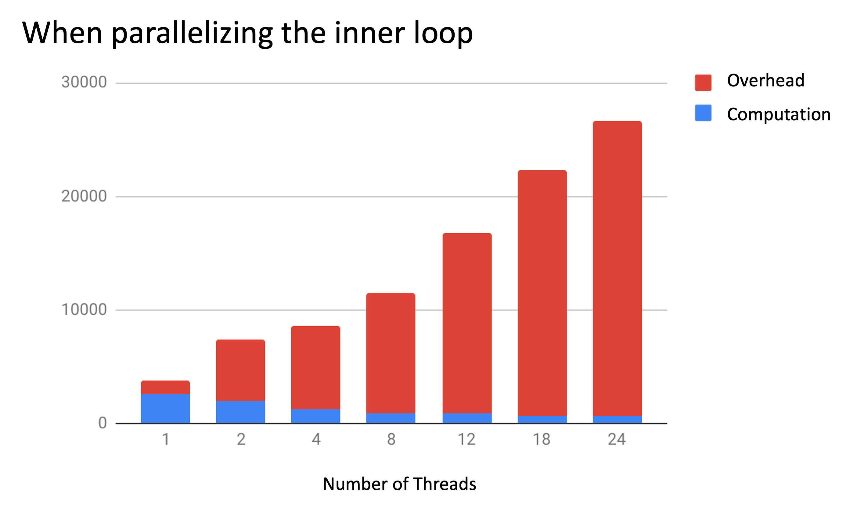
Blue is time spent actually computing, and red is overhead. Although computation time decreases steadily, overhead accounts for almost all the execution time, which is rather disastrous.
Next, the directive on the outer loop.
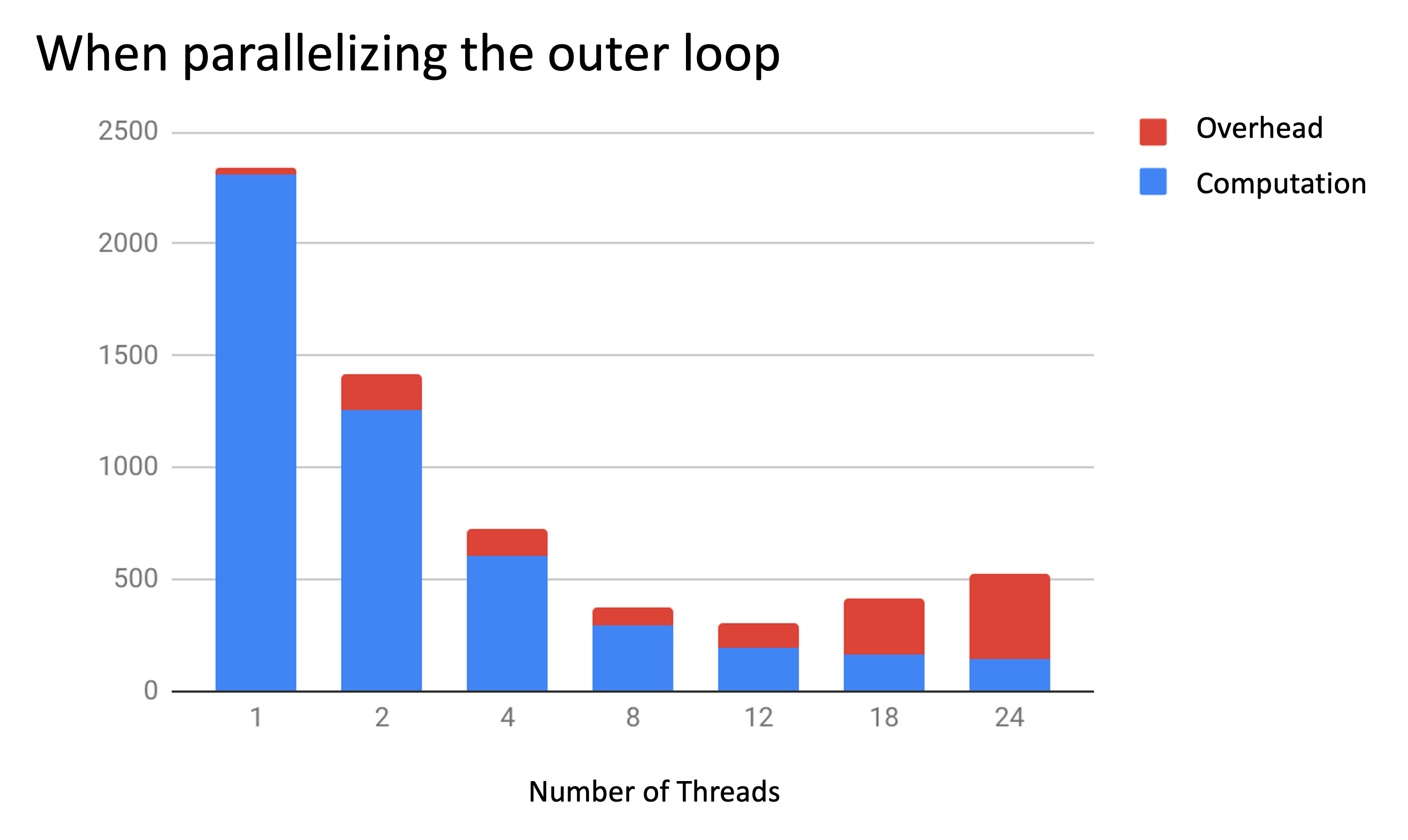
As before, blue is time spent actually computing, and red is overhead. Computation time decreases as the number of threads increases, but overhead grows along with it, so performance is best at 12 threads. Incidentally, 12 and 24 threads took almost the same amount of time earlier, but the 24-thread run was slower when the perf profile was recorded. Thread-parallel execution time fluctuates considerably when the computation is this light to begin with, so this much difference is within the margin of error.
Performance Evaluation
Section titled “Performance Evaluation”Parallelizing the outer loop worked reasonably well, but parallel efficiency was still only 27% with 24 threads. Judging only by the efficiency, there seems to be considerable room for improvement, which makes it tempting to try various tuning techniques. Before considering tuning, however, let us ask whether this number is actually good or bad, and, if it is bad, how far it is from the ideal.
This computation performs 20,000 steps in total. Since the serial computation takes 2,422 ms, each loop iteration takes about 120 ns. If it were parallelized ideally across 24 threads, only 5 ns would be available per loop. Even assuming that synchronizing 24 threads takes 5 ns on average, parallel efficiency would be only 50%. In reality, with 24 threads, computation takes an average of 7 ns and synchronization costs about 20 ns. With 12 threads, those figures are 9.7 ns and 5.7 ns, respectively. The machine used has two sockets with 12 cores each, so a little under 6 ns to synchronize the 12 cores within one CPU and 20 ns to synchronize all 24 cores across two CPUs both seem reasonable. This tells us that the real problem is simply that the computation is too light relative to the synchronization cost. Even if we work hard on optimizations such as loop fusion and loop fission, there does not appear to be much room for dramatic performance improvement.
When the inner loop is parallelized, the synchronization cost is multiplied further by the number of iterations of the outer loop. Here, L=128 and the loop executes L-2 times, so synchronization occurs 126 times as often as when the outer loop is parallelized. We can imagine that this will be quite painful.
What? The parallel efficiency is not good enough? Then increase the problem size!
So let us double the length of each side.
$ ./gs.out10032 [ms]conf000.dat
$ OMP_NUM_THREADS=12 ./gs_omp2.out12 threads 1104 [ms]conf000.dat
$ OMP_NUM_THREADS=24 ./gs_omp2.out24 threads 1023 [ms]conf000.dat
Because this is a two-dimensional system, the computation simply becomes four times heavier. The synchronization cost remains almost unchanged, so the relative parallel efficiency improves. In this case, parallel efficiency is 76% with 12 threads and 41% with 24 threads. It is easy to imagine that efficiency will rise as the problem size increases.
As a general rule, when synchronization costs become visible in thread parallelism, trying to eliminate those costs yields little reward for the effort. In that situation, reconsider the model being computed and perform a computation heavy enough to hide the synchronization cost. To repeat: if parallel efficiency is a problem, escape to weak scaling and beat it with problem size! Now that you have acquired the weapon of parallelization, rather than continuing to fight only the enemies you faced before acquiring it, it is more productive to seek enemies against which that weapon shines brightest.
I had originally intended to discuss OpenMP a little more seriously, including NUMA optimization and loop fusion, fission, and collapse, but honestly, it became too much trouble. This is only my personal impression, but with directive-based optimization it is difficult to see what the compiler is doing. It feels like scratching an itch through a boot, and I simply cannot bring myself to like it.
OpenMP has many constructs and can do a great variety of things. Many good OpenMP resources are available online; for example, I found the following Intel document easy to understand and recommend referring to it.
Introduction to OpenMP with the Intel Compiler
Professor Katagiri of Nagoya University has also prepared detailed lecture materials that are worth reading.
Advanced Topics in Computational Science and Engineering, Lecture 3: OpenMP Basics
Aside: Locks
Section titled “Aside: Locks”We wrote that the cost of synchronizing threads becomes a problem as the number of threads increases. Synchronization means “meeting up.” On a school trip, for example, students may have some free time, but before moving to the next place they must gather at a meeting point and confirm that everyone is present. Those who arrive first must wait for those who come later. This waiting time is the synchronization cost. That makes it sound as though CPUs would be idle while waiting for synchronization, but if we use the time command to run code in which the CPUs should be “idle” for nearly the entire synchronization wait, we get:
$ time OMP_NUM_THREADS=24 ./gs_omp1.out24 threads 24078 [ms]conf000.datOMP_NUM_THREADS=24 ./gs_omp1.out 573.12s user 1.72s system 2384% cpu 24.103 totalThis uses 2,384% CPU across 24 cores, showing that “almost every CPU core was busy.” Let us see what they were doing.
When run normally, the perf report command uses TUI mode. Let us use perf record on the extremely inefficient code that parallelized the “inner” loop.
OMP_NUM_THREADS=24 record ./gs_omp1.outAfter execution finishes, run perf report. You should see a screen like this.
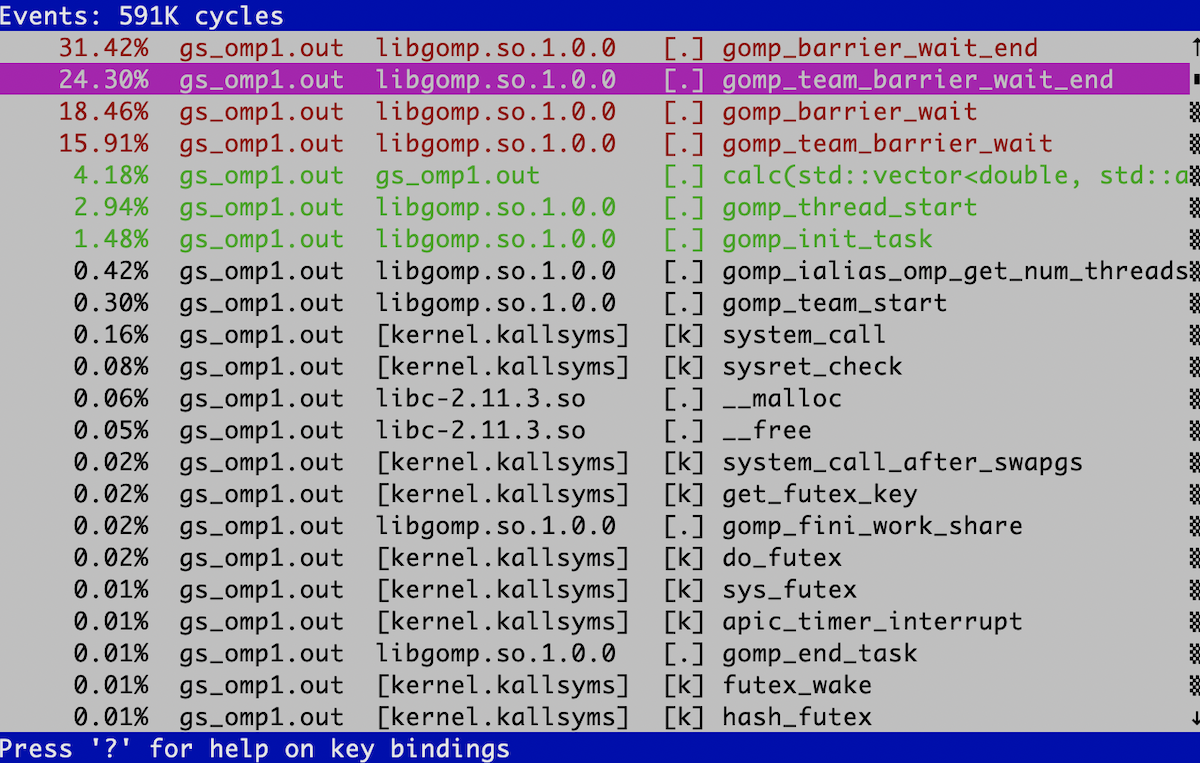
You can see functions with names obviously related to synchronization waits, such as gomp_barrier_wait_end and gomp_team_barrier_wait_end.
perf lets us look inside functions. First, let us inspect gomp_barrier_wait.
Use the up and down arrow keys to select the desired function and press Enter. Select the item labeled “Annotate gomp_barrier_wait.” You should see a screen like this.
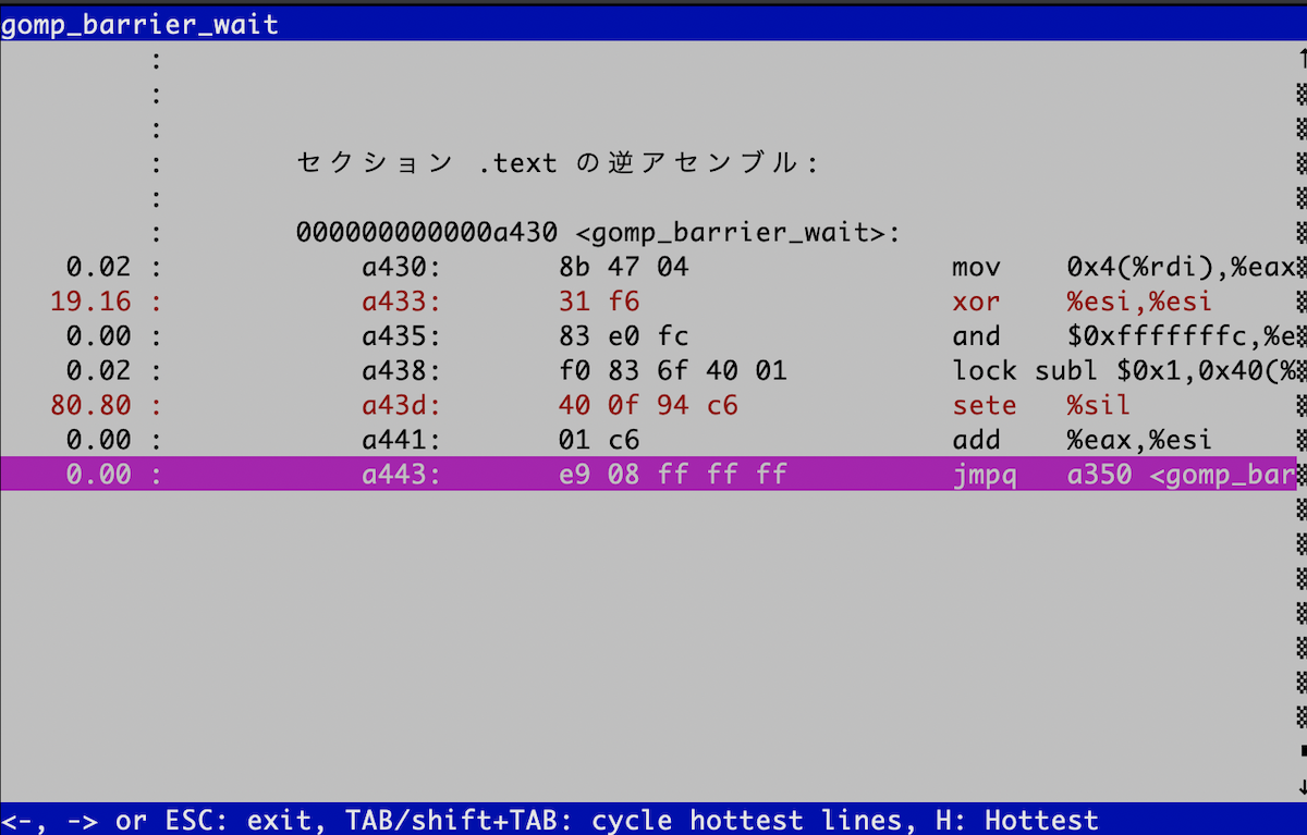
The code is very simple, but one instruction stands out: lock. In fact, lock is not an instruction but an instruction prefix. It is like a modifier saying, “Make the following instruction atomic.”
lock is followed by so-called read-modify-write instructions such as inc, xchg, and the subl shown here.
“Read-modify-write” means the sequence of reading something from memory, modifying it, and writing it back. Normally, this sequence is not atomic.
Atomic means indivisible: something that cannot be split apart. If the sequence is not atomic, another thread’s operation may intervene between its steps.
When this happens in multithreaded code, it can cause various problems. A commonly used example involves bank ATMs. Suppose we withdraw 10,000 yen from each of two ATMs at almost the same time from an account containing 1,000,000 yen.
Each ATM should perform three operations: read the account balance, subtract 10,000 yen (modify), and write back the remaining balance (990,000 yen).
But suppose ATM 1 and ATM 2 both read the account balance at the same time. Both believe that the balance is 1,000,000 yen. If each then performs the remaining operations of subtracting 10,000 yen and writing back the balance of 990,000 yen,
the balance will be 990,000 yen even though a total of 20,000 yen was withdrawn. To prevent such problems, CPUs that support multithreading provide hardware instructions that atomically perform the entire read-modify-write sequence. A compare-and-swap operation, commonly called a CAS instruction, is often used for this purpose, but we will not go into detail here.
Incidentally, methods for acquiring a safe lock without hardware support are also known, such as Peterson’s algorithm. These are generally slow, however, so hardware support is effectively essential for multithreaded implementations.
Now let us inspect the assembly for gomp_barrier_wait from above. We can simply run objdump on libgomp.so. The shared library should be somewhere in LD_LIBRARY_PATH, so find it there.
000000000000a430 <gomp_barrier_wait>: a430: 8b 47 04 mov 0x4(%rdi),%eax a433: 31 f6 xor %esi,%esi a435: 83 e0 fc and $0xfffffffc,%eax a438: f0 83 6f 40 01 lock subl $0x1,0x40(%rdi) a43d: 40 0f 94 c6 sete %sil a441: 01 c6 add %eax,%esi a443: e9 08 ff ff ff jmpq a350 <gomp_barrier_wait_end> a448: 0f 1f 84 00 00 00 00 nopl 0x0(%rax,%rax,1) a44f: 00We can see that it acquires a lock, decrements the value pointed to by a particular memory location, and then jumps to gomp_barrier_wait_end. Let us look there too.
According to perf, this loop was the “expensive” part.
a390: 44 8b 07 mov (%rdi),%r8d a393: 41 39 d0 cmp %edx,%r8d a396: 75 20 jne a3b8 <gomp_barrier_wait_end+0x68> a398: 48 83 c1 01 add $0x1,%rcx a39c: 48 39 f1 cmp %rsi,%rcx a39f: f3 90 pause a3a1: 75 ed jne a390 <gomp_barrier_wait_end+0x40>As you can probably tell, this loop monitors a location in memory, jumps to address a3b8 if a condition is satisfied, and otherwise returns to address a390 (the beginning of the excerpt).
In other words, threads are not idle while waiting for synchronization; they relentlessly repeat this loop until the condition is satisfied.
It is like continuously revving an engine while stopped at a red light.
This is why the CPU cores were somehow busy even though they appeared to be doing nothing but waiting for synchronization. Here they were spinning while “meeting up”; a method that spins in a loop to acquire a lock is called a spinlock. A spinlock is easy to implement if atomic read-modify-write instructions are available.
See the preceding Wikipedia article for details.
Incidentally, the CPU used in the K computer is the SPARC VIIIfx, which implements a hardware barrier.
I do not know the details of its implementation, but it is said to be more than ten times faster than software implementations such as spinlocks.
As we saw earlier, synchronization costs become visible in loops whose computations are light. Reducing synchronization costs with a hardware barrier makes even lighter computations easier to scale, which programmers appreciate.
A Real Example of Hybrid Parallelism
Section titled “A Real Example of Hybrid Parallelism”Now let us create hybrid-parallel code. That said, we already created an MPI-parallel version on Day 5, so all we need to do is add a single line, #pragma omp parallel for, to its computation routine.
Based on what we learned above, place the directive on the outer loop of the nested loop. The environment available to me had two sockets per node, 12 cores per socket, and could readily run jobs on up to 18 nodes,
so let us set the system size to about 324 to match it.
const int L = 9 * 36;This is convenient because it contains many factors of 2 and 3, which are the prime factors of 12 and 18.
While we are at it, let us measure the time and display the number of processes, number of threads, and computation time.
The number of executing threads can be obtained with omp_get_max_threads.
int num_threads = omp_get_max_threads();Any method of measuring time is fine, but here we will use std::chrono::system_clock::now.
const auto s = std::chrono::system_clock::now();// Some operation whose time we want to measureconst auto e = std::chrono::system_clock::now();const auto elapsed = std::chrono::duration_cast<std::chrono::milliseconds>(e - s).count();This stores a value in milliseconds in elapsed. The hybrid version of the reaction-diffusion equation solver created in this way is gs_hybrid.cpp.
https://github.com/kaityo256/sevendayshpc/blob/main/examples/day6/gs_hybrid.cpp
In the author’s environment, MPI is on the search path, so it can be compiled with the following options.
g++ -fopenmp -O3 -mavx2 gs_hybrid.cpp -lmpi -lmpi_cxxRunning it on my Mac with two processes x two threads produces the following output.
$ OMP_NUM_THREADS=2 mpiexec -np 2 ./a.out# Sytem Size = 324# 2 Process x 2 Threads# Domain = 2 x 12 2 4635 [ms]Let us benchmark it on the supercomputer available to us. Its processors are Intel(R) Xeon(R) CPU E5-2680 v3 @ 2.50GHz, with two sockets of 12 cores each per node. First, on one node, here are the results starting from one process and one thread, then increasing only the number of threads through 2, 3, 4, 6, …, and separately increasing only the number of processes through 2, 3, 4, 6, …
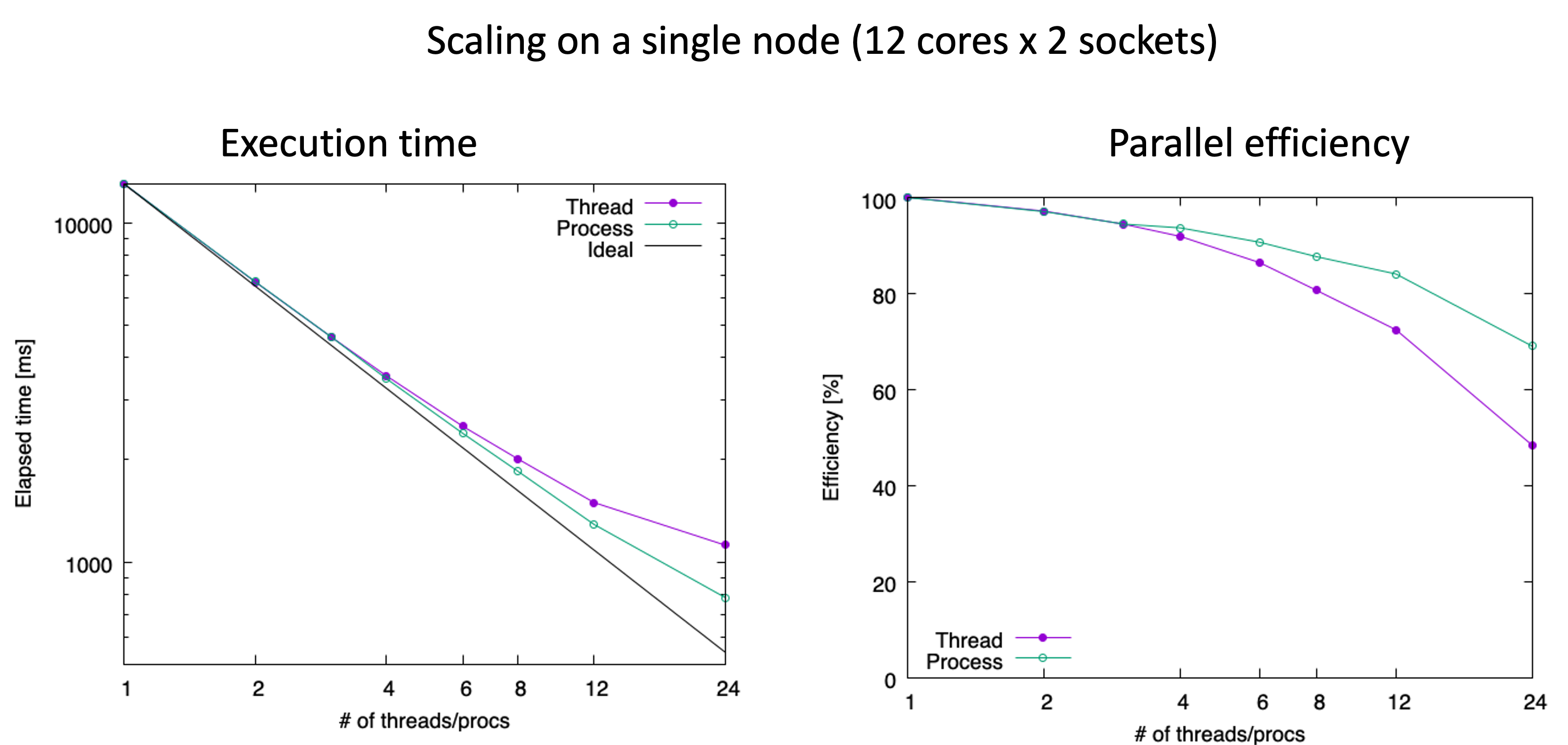
The left graph shows execution time on log-log axes, and the right shows parallel efficiency with a logarithmic horizontal axis. We can see that increasing the number of processes—in other words, using flat MPI—provides better execution efficiency. With 24 processes, the computation is 16.6 times faster than serial, corresponding to about 70% parallel efficiency. Running entirely with thread parallelism is not especially bad either, but with 24 threads it is only 11.6 times faster than serial, for a parallel efficiency of 48%, below 50%. Because MPI has the added work of creating and copying buffers, it might seem likely to be slower than multithreading, but flat MPI was faster in this case.
Next, let us cross node boundaries. We will compute on 18 nodes. Each node has two sockets x 12 cores, or 24 cores total, so there are 18x24=432 CPU cores altogether. Keeping the entire program at 432 threads, let us vary the number of processes. With flat MPI, for example, there is one thread per process, so the maximum is 432 processes. If each node is filled with 24 threads, the minimum process count is 18 processes with 24 threads each. The following graph plots the number of processes on the horizontal axis and execution time on the vertical axis.
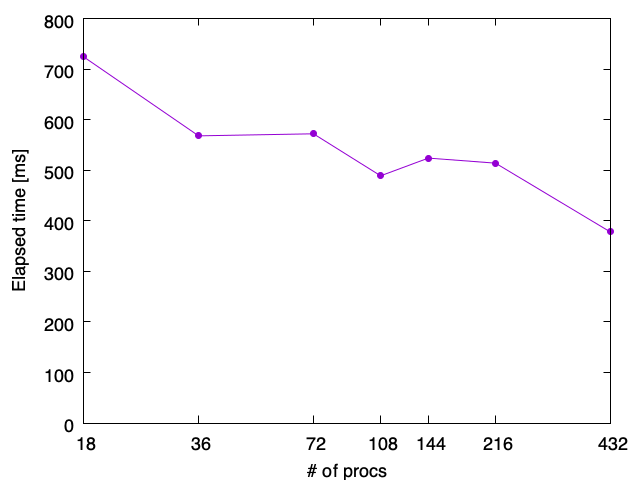
The horizontal axis uses a logarithmic scale. Every run uses 432 threads in total; the only difference is how many threads are grouped into each process. Here, the 432-process computation—that is, the flat-MPI computation in which each process has only one thread—was fastest.
As a general rule, there is an optimal ratio of processes to threads, and the only way to know which is fastest is to try it. In the author’s experience, however, flat MPI is often fastest when the computation is very simple but still reasonably substantial. That said, the author is not very experienced with thread parallelization, so perhaps someone skilled in OpenMP could tune the preceding code and make the hybrid version faster. Please experiment with it. Pull requests reporting findings such as “this made it faster” or “this was the problem” are welcome.