Day 3: Embarrassingly Parallel Computing

Suppose, for example, that you have 100 image files and want to resize all of them. Because the individual tasks have no dependencies whatsoever, there is no problem with running them all at once. Running them with 100-way parallelism should therefore make the job 100 times faster. Parallelization in which parallel tasks have no dependencies or exchange of information is called embarrassingly parallel computing. It is also sometimes called trivial parallelization. Although embarrassingly parallel work is sometimes looked down upon precisely because it is so easy to parallelize, it achieves 100% parallel efficiency and therefore makes the most effective possible use of computing resources. It is consequently very important. After all, you cannot tackle non-trivial parallelism until you can first handle embarrassingly parallel work. Even this skill alone gives you an overwhelming advantage over someone who cannot do it. In this chapter, we will begin by learning how to implement embarrassingly parallel programs.

Embarrassingly Parallel Example 1: Pi

We will begin with an example commonly used in embarrassingly parallel computing: increasing the number of samples through parallelization. As a standard exercise, let us estimate pi using the Monte Carlo method.

Write the following code and save it as calc_pi.cpp.

#include <cstdio>
#include <random>
#include <algorithm>

const int TRIAL = 100000;

double calc_pi(const int seed) {
  std::mt19937 mt(seed);
  std::uniform_real_distribution<double> ud(0.0, 1.0);
  int n = 0;
  for (int i = 0; i < TRIAL; i++) {
    double x = ud(mt);
    double y = ud(mt);
    if (x * x + y * y < 1.0) n++;
  }
  return 4.0 * static_cast<double>(n) / static_cast<double>(TRIAL);
}

int main(void) {
  double pi = calc_pi(0);
  printf("%f\n", pi);
}

Notice that the function calc_pi(const int seed), called from main, has been deliberately written to accept only a random-number seed.

Compile and run it normally.

$ g++ calc_pi.cpp
$ ./a.out
3.145000

After 100,000 trials, we obtain the estimate 3.145000 for pi. Now let us parallelize it. The procedure is straightforward.

1. Include mpi.h.
2. Add MPI_Init and MPI_Finalize at the beginning and end of main. Since MPI_Init requires argc and argv, give main its full argument list.
3. Obtain the rank with MPI_Comm_rank.
4. Use the rank as the random-number seed.
5. Call calc_pi as before.

Create a file named calc_pi_mpi.cpp with these changes.

#include <cstdio>
#include <random>
#include <algorithm>
#include <mpi.h>

const int TRIAL = 100000;

double calc_pi(const int seed) {
  std::mt19937 mt(seed);
  std::uniform_real_distribution<double> ud(0.0, 1.0);
  int n = 0;
  for (int i = 0; i < TRIAL; i++) {
    double x = ud(mt);
    double y = ud(mt);
    if (x * x + y * y < 1.0) n++;
  }
  return 4.0 * static_cast<double>(n) / static_cast<double>(TRIAL);
}

int main(int argc, char **argv) {
  MPI_Init(&argc, &argv);
  int rank;
  MPI_Comm_rank(MPI_COMM_WORLD, &rank);
  double pi = calc_pi(rank);
  printf("%d: %f\n", rank, pi);
  MPI_Finalize();
}

We also made each process print its own rank alongside its estimate of pi. The output is as follows.

$ mpic++ calc_pi_mpi.cpp
$ mpirun -np 4 --oversubscribe ./a.out
0: 3.145000
1: 3.142160
3: 3.144200
2: 3.146720

$ mpirun -np 4 --oversubscribe ./a.out
0: 3.145000
2: 3.146720
3: 3.144200
1: 3.142160

The --oversubscribe option permits launching more processes than there are logical CPU cores. These results show that:

1. The output order changes on every run.
2. The estimate associated with a given rank does not change.

Use the time command to check that the calculation really is running in parallel.

$ time ./a.out
0: 3.145000
./a.out  0.04s user 0.01s system 57% cpu 0.086 total

$ time mpirun -np 4 --oversubscribe ./a.out
2: 3.146720
3: 3.144200
1: 3.142160
0: 3.145000
mpirun -np 4 --oversubscribe ./a.out  0.24s user 0.08s system 240% cpu 0.135 total

The CPU utilization was 57% for the serial run, but rose above 100% to 240% with four processes. This example finishes too quickly to make the effect easy to see, but if you increase TRIAL so that execution takes longer and inspect the system with top while it is running, you can confirm that the program is indeed executing in parallel.

PID    COMMAND      %CPU TIME     #TH   #WQ  #PORT MEM    PURG   CMPRS  PGRP
45163  a.out        92.1 00:12.44 3/1   0    15    2612K  0B     0B     45163
45165  a.out        91.8 00:12.48 3/1   0    15    2620K  0B     0B     45165
45164  a.out        91.5 00:12.42 3/1   0    15    2608K  0B     0B     45164
45162  a.out        89.1 00:12.47 3/1   0    15    2620K  0B     0B     45162

Because we launched four processes, four processes with PIDs 45162 through 45165 are running. Parallelization that uses additional computing resources to obtain more samples for a statistical average is called sample parallelism.

An Embarrassingly Parallel Template

The main function in the preceding parallel program, calc_pi_mpi.cpp, looked like this.

int main(int argc, char **argv) {
  MPI_Init(&argc, &argv);
  int rank;
  MPI_Comm_rank(MPI_COMM_WORLD, &rank);
  double pi = calc_pi(rank);
  printf("%d: %f\n", rank, pi);
  MPI_Finalize();
}

The actual computation is entirely contained in calc_pi(rank), a function that accepts the rank—the sequential number assigned to an MPI process—and changes its behavior according to that number. An embarrassingly parallel program can therefore use the following template.

#include <cstdio>
#include <mpi.h>

void func(const int rank){
  // Fill this in
}

int main(int argc, char **argv) {
  MPI_Init(&argc, &argv);
  int rank;
  MPI_Comm_rank(MPI_COMM_WORLD, &rank);
  func(rank);
  MPI_Finalize();
}

You can parallelize almost anything—file processing, rendering, machine learning, and so on—simply by replacing the body of func. Someone may object that this can be done with threads without using MPI. There is, however, a major difference between multithreaded programming with OpenMP or std::thread and multiprocess programming with MPI: whether execution can span multiple nodes. In general, multithreaded programs cannot span nodes. A single program is therefore limited to the computing resources of one node. An MPI program, by contrast, can use any number of nodes.

If you wish, the preceding pi program can be run on tens of thousands of nodes. In other words, now that you can write this code, you are a supercomputer programmer regardless of what anyone says. This text is titled Become an HPC Programmer in Seven Days!, but you have already become one on Day 3.

Embarrassingly Parallel Example 2: Processing Many Files

As another example, consider processing a large number of files. Suppose you have 1,000 files, each of which takes five minutes to process. Processing them normally would take 5,000 minutes. Even if you have an eight-core local machine and parallelize the work perfectly, it would still take 625 minutes—more than ten hours.

If you have access to a supercomputer or cluster capable of running MPI jobs, however, the work can finish in no time. Suppose, for example, that you can use ten nodes, each containing two sockets with eight CPU cores per socket. With effective parallelization, the task would finish in just over 30 minutes. Processing large numbers of files is a common situation even outside supercomputing, so it is useful to know how to handle it with embarrassingly parallel computing.

For simplicity, suppose the files are numbered sequentially from file000.dat through file999.dat. When using $N$ processes, each process can handle the files whose index modulo $N$ equals its rank. Parallelization that independently processes different inputs in this way is called parameter parallelism. For example, processing 100 files with 16 processes might look like this.

#include <cstdio>
#include <mpi.h>

void process_file(const int index, const int rank) {
  printf("Rank=%03d File=%03d\n", rank, index);
}

int main(int argc, char **argv) {
  MPI_Init(&argc, &argv);
  int rank;
  const int procs = 16;
  MPI_Comm_rank(MPI_COMM_WORLD, &rank);
  const int max_file = 100;
  for (int i = rank; i < max_file; i += procs) {
    process_file(i, rank);
  }
  MPI_Finalize();
}

The number of files aside, hard-coding the number of processes is undesirable. An MPI program lets you choose the process count freely at run time, and recompiling whenever you change it would be inconvenient. MPI therefore provides MPI_Comm_size, which obtains the total number of processes at run time. Its usage resembles MPI_Comm_rank:

int procs;
MPI_Comm_size(MPI_COMM_WORLD, &procs)

After this call, procs contains the number of processes. Using it, the preceding code can be written as follows (processfiles.cpp).

#include <cstdio>
#include <mpi.h>

void process_file(const int index, const int rank) {
  printf("Rank=%03d File=%03d\n", rank, index);
}

int main(int argc, char **argv) {
  MPI_Init(&argc, &argv);
  int rank;
  int procs;
  MPI_Comm_rank(MPI_COMM_WORLD, &rank);
  MPI_Comm_size(MPI_COMM_WORLD, &procs);
  const int max_file = 100;
  for (int i = rank; i < max_file; i += procs) {
    process_file(i, rank);
  }
  MPI_Finalize();
}

Now you only need to implement process_file, and the file processing will be parallelized across nodes. If the work does not need to span nodes—that is, if shared-memory parallelism is sufficient—you can process it without writing an MPI program, for example by using Makefile’s parallel execution feature. To repeat the crucial point, MPI’s advantage is that a parallel program can span nodes.

Embarrassingly Parallel Example 3: Statistical Processing

At the beginning of this chapter, we estimated pi using embarrassingly parallel computing. With $N$ processes, we obtain $N$ estimates and could process them statistically afterward. Since we are already using MPI, however, let us perform the statistical processing with MPI as well. Suppose each process obtains an estimate $x_i$ of pi. The mean is

$$\bar{x} = \frac{1}{N} \sum x_i$$

and the unbiased variance $\sigma^2$ is

$$\sigma^2 = \frac{1}{n-1} \sum (x_i)^2 - \frac{n}{n-1} \bar{x}^2.$$

Thus, once we know the sum of the estimates $x_i$ and the sum of their squares $x_i^2$, we can calculate the expected value and standard deviation.

In MPI, a global sum can be computed with MPI_Allreduce.

double pi =  calc_pi(rank);
double pi_sum = 0.0;
MPI_Allreduce(&pi, &pi_sum, 1, MPI_DOUBLE, MPI_SUM, MPI_COMM_WORLD);

The arguments specify, in order: the variable to sum, the variable that receives the result, the number of values, the value type, the operation to perform, and the communicator. Although we sum only one value here, you can pass an array to reduce multiple values in one call. MPI can also perform products and logical operations, not just sums.

The following program, calc_pi_reduce.cpp, sums both the estimate pi and its square pi2 = pi*pi, then calculates the expected value and standard deviation directly from their definitions.

#include <cstdio>
#include <random>
#include <algorithm>
#include <cmath>
#include <mpi.h>

const int TRIAL = 100000;

double calc_pi(const int seed) {
  std::mt19937 mt(seed);
  std::uniform_real_distribution<double> ud(0.0, 1.0);
  int n = 0;
  for (int i = 0; i < TRIAL; i++) {
    double x = ud(mt);
    double y = ud(mt);
    if (x * x + y * y < 1.0) n++;
  }
  return 4.0 * static_cast<double>(n) / static_cast<double>(TRIAL);
}

int main(int argc, char **argv) {
  MPI_Init(&argc, &argv);
  int rank;
  int procs;
  MPI_Comm_rank(MPI_COMM_WORLD, &rank);
  MPI_Comm_size(MPI_COMM_WORLD, &procs);
  double pi = calc_pi(rank);
  double pi2 = pi * pi;
  double pi_sum = 0.0;
  double pi2_sum = 0.0;
  printf("%f\n", pi);
  MPI_Allreduce(&pi, &pi_sum, 1, MPI_DOUBLE, MPI_SUM, MPI_COMM_WORLD);
  MPI_Allreduce(&pi2, &pi2_sum, 1, MPI_DOUBLE, MPI_SUM, MPI_COMM_WORLD);
  double pi_ave = pi_sum / procs;
  double pi_var = pi2_sum / (procs - 1) - pi_sum * pi_sum / procs / (procs - 1);
  double pi_stdev = sqrt(pi_var);
  MPI_Barrier(MPI_COMM_WORLD);
  if (rank == 0) {
    printf("pi = %f +- %f\n", pi_ave, pi_stdev);
  }
  MPI_Finalize();
}

The final MPI_Barrier instructs every process to wait at that point. MPI_Allreduce shares information among all processes, and rank 0 then represents them by printing the statistics at the end. Here is an example run.

$ mpic++ calc_pi_reduce.cpp
$ mpirun --oversubscribe -np 4  ./a.out
3.144200
3.142160
3.146720
3.145000
pi = 3.144520 +- 0.001892

$ mpirun --oversubscribe -np 8  ./a.out
3.145000
3.142160
3.144200
3.144080
3.139560
3.146720
3.139320
3.136040
pi = 3.142135 +- 0.003565

Four processes produce four estimates, while eight processes produce eight; the mean and standard deviation appear last. Try entering the values into Excel or Google Sheets and verify that they were calculated correctly. Incidentally, we would expect more processes to yield a smaller standard deviation, but perhaps because the random-number seeds were poorly chosen, these data are biased. If this concerns you, feel free to improve the program.

Parallel Efficiency

After parallelizing a program, you will want to know how effective the parallelization is compared with the original serial version. Parallel efficiency expresses that effectiveness. Even if you are not personally curious, once you parallelize something, someone will inevitably ask, “What is the parallel efficiency?” I think it is better at first to have fun without worrying too much about efficiency, but you should still understand the concept.

Parallelization uses more computing resources either to finish the same task sooner or to run a larger task. Scaling describes how efficiently a program benefits as computing resources increase. Ideally, when we devote $N$ times as many resources to the same task, it should finish in $1/N$ of the time. This is called strong scaling. Conversely, if we keep the task size per unit of computing resource fixed, a task using $N$ times the resources—and therefore $N$ times the total problem size—should still finish in the same amount of time. This is called weak scaling. Achieving good strong-scaling efficiency is generally harder than achieving good weak-scaling efficiency.

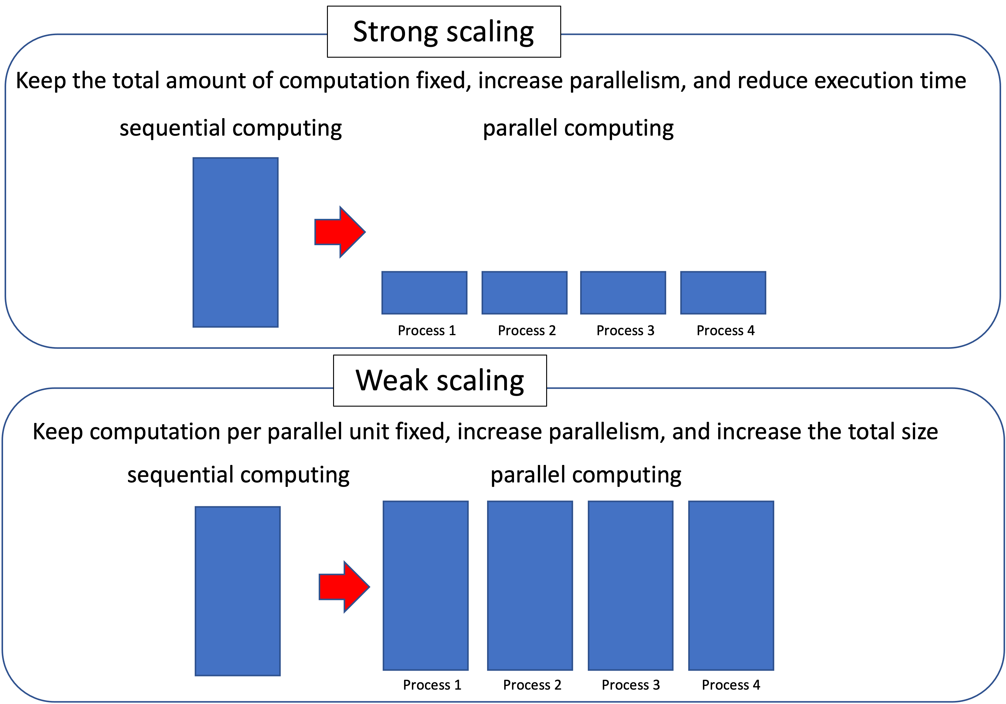
First, let us define strong-scaling efficiency. The unit of parallelism may be a process or a thread, but for now we will consider process parallelism; parallel efficiency for threads is defined in exactly the same way. Suppose a task finishes in time $T_1$ before parallelization—that is, when run by one process. If the same-size task takes time $T_N$ on $N$ processes, the parallel efficiency $\alpha$ is defined as

$$\alpha = \frac{T_1}{N T_N}.$$

For example, if a job that takes ten seconds on one process finishes in one second on ten processes, its parallel efficiency is 1 (100%). If it takes two seconds on ten processes, its parallel efficiency is 0.5 (50%).

In weak scaling, the task size per process remains fixed. As the number of processes grows, the total problem size therefore grows proportionally. If both problem size and process count increase by a factor of ten, for example, we ideally want the execution time to remain unchanged. We define the efficiency to be 1 in that ideal case. Suppose a certain task finishes in time $T_1$ on one process, while a task $N$ times as large finishes in time $T_N$ on $N$ processes. The parallel efficiency $\alpha$ is then

$$\alpha = \frac{T_1}{T_N}.$$

For example, suppose a task finishes in 12 seconds on one process. If a task ten times as large takes 16 seconds on ten processes, the parallel efficiency is $12/16 = 0.75$, or 75%.

In short, a smaller post-parallelization execution time $T_N$ is better—that is, it means higher parallel efficiency—so remember that $T_N$ belongs in the denominator. Strong scaling has the factor $N$, whereas weak scaling does not. If you think through the ideal cases, you can quickly recall which formula is which.

The Difference Between Sample and Parameter Parallelism

In Day 3, we introduced sample parallelism and parameter parallelism as forms of embarrassingly parallel computing. Sample parallelism uses computing resources to obtain more samples for a statistical average. Parameter parallelism uses them to process different parameter values. We used file processing as an example of parameter parallelism, but another typical example would be studying a system’s temperature dependence by running ten temperatures in parallel.

Both sample and parameter parallelism are forms of weak scaling. Unless the execution times of the individual tasks vary greatly, they can maintain nearly ideal parallel efficiency even at very large scales. There is, however, an important difference: 100 times the resources allow parameter parallelism to process 100 times as many parameter values, but give sample parallelism only ten times the statistical precision. This is because sampling accuracy improves only as the square root of the number of samples.

Consequently, even when parallel efficiency is nearly 100%, devoting enormous computing resources to sample averaging may not be very effective. Before spending 100 times the resources merely to gain one decimal digit of accuracy, investigate whether a more efficient method exists. Similarly, combining multiple dimensions in a parameter sweep can make the number of points to examine extremely large. Exhaustively exploring every combination in fine detail with parameter parallelism is then inefficient. Parameter parallelism is useful for quickly finding a promising region; after locating the area worth investigating, use another method to examine it in detail.