Day 5: Two-Dimensional Reaction-Diffusion Equation

On Day 4, we parallelized the one-dimensional diffusion equation using domain decomposition. The same idea applies to any short-range interaction model, although two and three dimensions are somewhat more complicated. The heat equation also tends toward a final steady state, which makes it less exciting to simulate. We will therefore study a two-dimensional reaction-diffusion equation: it is easy to solve with finite differences and produces interesting results.

Reaction-Diffusion Equations

A reaction-diffusion system combines diffusion equations with a dynamical system and produces a wide variety of patterns. Try an image search for “reaction-diffusion system.” Such equations can explain patterns seen on living organisms.

Many reaction-diffusion equations exist. Here we consider the following system, known as the Gray-Scott model.

\frac{\partial u}{\partial t} = D_u \Delta u + u^2 v - (F+k)u

\frac{\partial v}{\partial t} = D_v \Delta v - u^2 v + F(1-v)

These equations model a chemical reaction between substances $U$ and $V$ . $U$ is called the activator and $V$ the inhibitor. If their concentrations are $u$ and $v$ , respectively, the equations show that $U$ is not produced where $V$ is abundant. $D_u$ and $D_v$ are diffusion coefficients; we choose $D_v/D_u = 2$ , so $V$ diffuses more readily. Let us simulate these equations.

Incidentally, our $U$ and $V$ appear to be reversed relative to the notation most widely used. The author noticed only after finishing the program, so we apologize but retain the notation here.

Serial Version

First, define a function laplacian that returns the Laplacian at a point. Using central differences, it is the difference from the four neighboring points and can be written as follows.

double laplacian(int ix, int iy, vd &s) {
  double ts = 0.0;
  ts += s[ix - 1 + iy * L];
  ts += s[ix + 1 + iy * L];
  ts += s[ix + (iy - 1) * L];
  ts += s[ix + (iy + 1) * L];
  ts -= 4.0 * s[ix + iy * L];
  return ts;
}

Also define a function that calculates the dynamical-system terms for $u$ and $v$ .

double calcU(double tu, double tv) {
  return tu * tu * tv - (F + k) * tu;
}

double calcV(double tu, double tv) {
  return -tu * tu * tv + F * (1.0 - tv);
}

When evaluating finite differences at step $t+1$ , we use physical quantities from step $t$ . Updating the values for $t$ in place would mix values from $t$ and $t+1$ during the same sweep and produce incorrect results. In the one-dimensional diffusion equation, we avoided this by copying all values at $t$ to another region before calculating $t+1$ —a shortcut whose copying overhead becomes substantial in two dimensions.

Instead, provide two arrays for each physical quantity and alternate between them on even and odd steps. Alongside u, for example, define u2. On an even step, calculate u from u2; on an odd step, calculate u2 from u.

The function calc, which advances the system by one step, can therefore be written as follows.

void calc(vd &u, vd &v, vd &u2, vd &v2) {
  for (int iy = 1; iy < L - 1; iy++) {
    for (int ix = 1; ix < L - 1; ix++) {
      double du = 0;
      double dv = 0;
      const int i = ix + iy * L;
      du = Du * laplacian(ix, iy, u);
      dv = Dv * laplacian(ix, iy, v);
      du += calcU(u[i], v[i]);
      dv += calcV(u[i], v[i]);
      u2[i] = u[i] + du * dt;
      v2[i] = v[i] + dv * dt;
    }
  }
}

In the Gray-Scott system, a pattern spreads from an initial seed, so we must plant one first.

void init(vd &u, vd &v) {
  int d = 3;
  for (int i = L / 2 - d; i < L / 2 + d; i++) {
    for (int j = L / 2 - d; j < L / 2 + d; j++) {
      u[j + i * L] = 0.7;
    }
  }
  d = 6;
  for (int i = L / 2 - d; i < L / 2 + d; i++) {
    for (int j = L / 2 - d; j < L / 2 + d; j++) {
      v[j + i * L] = 0.9;
    }
  }
}

This code places initial values in 6x6 and 12x12 regions of $u$ and $v$ , respectively, at the center of the system.

Based on the above, the main function that performs time evolution is as follows.

int main() {
  const int V = L * L;
  vd u(V, 0.0), v(V, 0.0);
  vd u2(V, 0.0), v2(V, 0.0);
  init(u, v);
  for (int i = 0; i < TOTAL_STEP; i++) {
    if (i & 1) {
      calc(u2, v2, u, v);
    } else {
      calc(u, v, u2, v2);
    }
    if (i % INTERVAL == 0) save_as_dat(u);
  }
}

Notice that, as described above, the two arrays alternate between even and odd steps.

save_as_dat saves the array under a sequentially numbered filename each time it is called.

The complete program is shown below (gs.cpp).

#include <cstdio>
#include <iostream>
#include <vector>
#include <fstream>

const int L = 128;
const int TOTAL_STEP = 20000;
const int INTERVAL = 200;
const double F = 0.04;
const double k = 0.06075;
const double dt = 0.2;
const double Du = 0.05;
const double Dv = 0.1;

typedef std::vector<double> vd;

void init(vd &u, vd &v) {
  int d = 3;
  for (int i = L / 2 - d; i < L / 2 + d; i++) {
    for (int j = L / 2 - d; j < L / 2 + d; j++) {
      u[j + i * L] = 0.7;
    }
  }
  d = 6;
  for (int i = L / 2 - d; i < L / 2 + d; i++) {
    for (int j = L / 2 - d; j < L / 2 + d; j++) {
      v[j + i * L] = 0.9;
    }
  }
}

double calcU(double tu, double tv) {
  return tu * tu * tv - (F + k) * tu;
}

double calcV(double tu, double tv) {
  return -tu * tu * tv + F * (1.0 - tv);
}

double laplacian(int ix, int iy, vd &s) {
  double ts = 0.0;
  ts += s[ix - 1 + iy * L];
  ts += s[ix + 1 + iy * L];
  ts += s[ix + (iy - 1) * L];
  ts += s[ix + (iy + 1) * L];
  ts -= 4.0 * s[ix + iy * L];
  return ts;
}

void calc(vd &u, vd &v, vd &u2, vd &v2) {
  for (int iy = 1; iy < L - 1; iy++) {
    for (int ix = 1; ix < L - 1; ix++) {
      double du = 0;
      double dv = 0;
      const int i = ix + iy * L;
      du = Du * laplacian(ix, iy, u);
      dv = Dv * laplacian(ix, iy, v);
      du += calcU(u[i], v[i]);
      dv += calcV(u[i], v[i]);
      u2[i] = u[i] + du * dt;
      v2[i] = v[i] + dv * dt;
    }
  }
}

void save_as_dat(vd &u) {
  static int index = 0;
  char filename[256];
  sprintf(filename, "conf%03d.dat", index);
  std::cout << filename << std::endl;
  std::ofstream ofs(filename, std::ios::binary);
  ofs.write((char *)(u.data()), sizeof(double)*L * L);
  index++;
}

int main() {
  const int V = L * L;
  vd u(V, 0.0), v(V, 0.0);
  vd u2(V, 0.0), v2(V, 0.0);
  init(u, v);
  for (int i = 0; i < TOTAL_STEP; i++) {
    if (i & 1) {
      calc(u2, v2, u, v);
    } else {
      calc(u, v, u2, v2);
    }
    if (i % INTERVAL == 0) save_as_dat(u);
  }
}

Compile and run it.

$ g++ -O3 gs.cpp
$ time ./a.out
conf000.dat
conf001.dat
conf002.dat
(snip)
conf097.dat
conf098.dat
conf099.dat
./a.out  1.61s user 0.03s system 96% cpu 1.697 total

Each output file (*.dat) contains L*L double-precision values. Create a Ruby script that reads them and writes a PNG image.

image.rb

require "cairo"
require "pathname"

def convert(datfile)
  puts datfile
  buf = File.binread(datfile).unpack("d*")
  l = Math.sqrt(buf.size).to_i
  m = 4
  size = l * m

  surface = Cairo::ImageSurface.new(Cairo::FORMAT_RGB24, size, size)
  context = Cairo::Context.new(surface)
  context.set_source_rgb(1, 1, 1)
  context.rectangle(0, 0, size, size)
  context.fill

  l.times do |x|
    l.times do |y|
      u = buf[x + y * l]
      context.set_source_rgb(0, u, 0)
      context.rectangle(x * m, y * m, m, m)
      context.fill
    end
  end
  pngfile = Pathname(datfile).sub_ext(".png").to_s
  surface.write_to_png(pngfile)
end

`ls *.dat`.split(/\n/).each do |f|
  convert(f)
end

Process all files at once with this command.

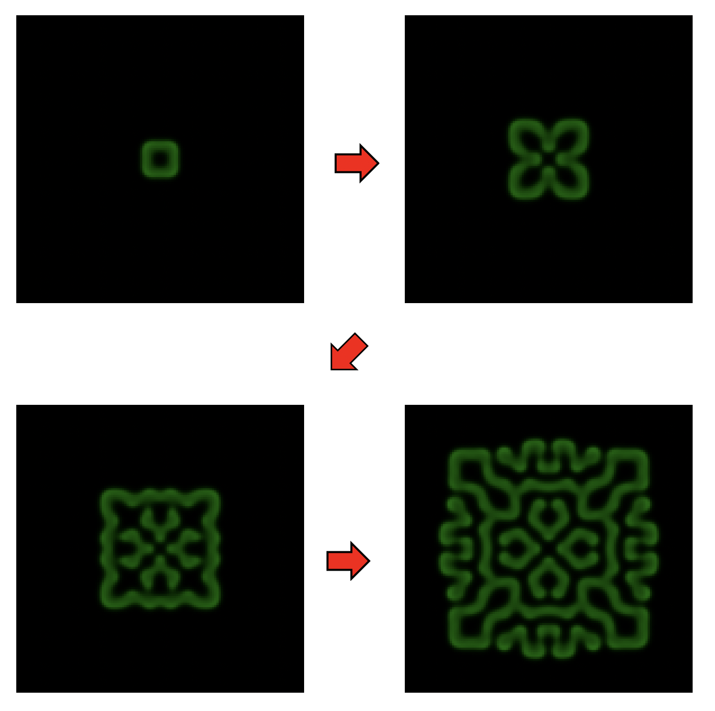
$ ruby image.rb
conf000.dat
conf001.dat
conf002.dat
(snip)
conf097.dat
conf098.dat
conf099.dat

This produces images like the following.

Result of the reaction-diffusion simulation

Parallelization Step 1: Preparing for Communication

We will now parallelize the reaction-diffusion equation with two-dimensional domain decomposition. A crucial rule is: do not test a communication algorithm for the first time in production code. First write a small program containing only the planned communication algorithm, and verify that it communicates exactly as intended. The real data are double-precision values, but we will experiment with integers.

Before writing communication code, establish the basic domain-decomposition setup: how the full domain is divided and which portion each process owns.

Suppose an $L\times L$ grid is divided among procs processes. We want to minimize the halo boundaries, so four processes should form a 2x2 grid, 24 processes a 6x4 grid, and so on. This requires factoring the process count into numbers as close as possible. MPI provides MPI_Dims_create for this purpose. For a two-dimensional decomposition, with the process count in procs, call it as follows.

  int d2[2] = {};
  MPI_Dims_create(procs, 2, d2);

The numbers of divisions are returned in d2[0] and d2[1]. For a three-dimensional decomposition, specify three dimensions and supply a three-element array:

  int d3[3] = {};
  MPI_Dims_create(procs, 3, d3);

Be aware that Open MPI’s MPI_Dims_create can behave somewhat unexpectedly. A two-dimensional division of nine processes should ideally return 3x3, but it may return 9x1. Intel MPI and SGI MPT correctly return 3x3, so this appears implementation-dependent. If it matters, write your own factorization routine.

Let us divide procs processes into a GX*GY grid. Each process then owns L/GX sites horizontally and L/GY vertically. When an 8x8 system is parallelized over four processes, for example, each process owns a 4x4 region, but needs one extra row or column on every side for halos, so it stores 6x6 values in total.

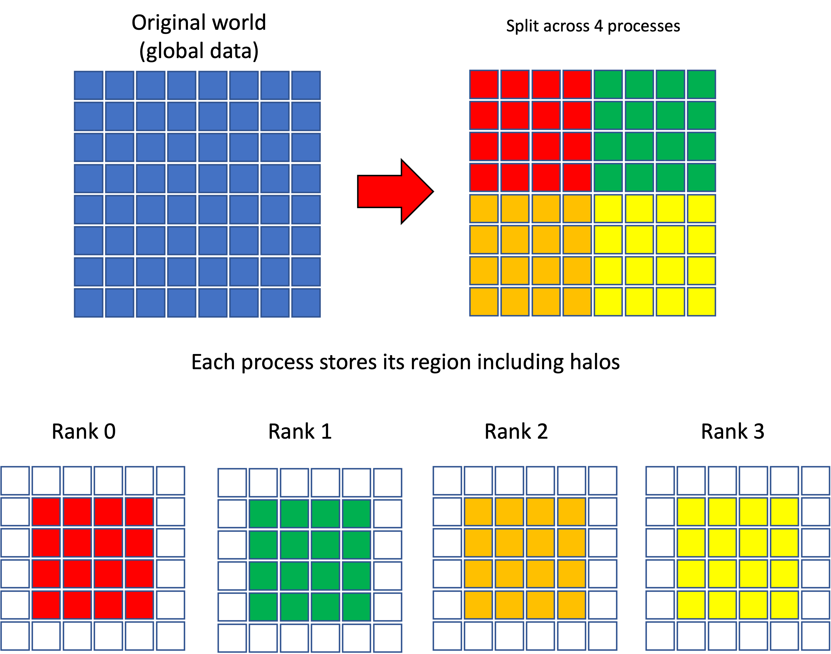
Halo regions used for communication

Each process also needs to know which position it owns and the size of its region. Collect this information together with the rank and total process count in a structure named MPIinfo. The following fields should be sufficient.

struct MPIinfo {
  int rank;  // Rank
  int procs; // Total number of processes
  int GX, GY; // Process-grid dimensions (GX*GY=procs)
  int local_grid_x, local_grid_y; // Position owned by this process
  int local_size_x, local_size_y; // Size of the owned region (excluding halos)
};

Define setup_info to initialize the members of MPIinfo.

void setup_info(MPIinfo &mi) {
  int rank = 0;
  int procs = 0;
  MPI_Comm_rank(MPI_COMM_WORLD, &rank);
  MPI_Comm_size(MPI_COMM_WORLD, &procs);
  int d2[2] = {};
  MPI_Dims_create(procs, 2, d2);
  mi.rank = rank;
  mi.procs = procs;
  mi.GX = d2[0];
  mi.GY = d2[1];
  mi.local_grid_x = rank % mi.GX;
  mi.local_grid_y = rank / mi.GX;
  mi.local_size_x = L / mi.GX;
  mi.local_size_y = L / mi.GY;
}

Declare the data held by each process as std::vector<int> local_data. Including the halo regions, its size is as follows.

  MPIinfo mi;
  setup_info(mi);
  std::vector<int> local_data((mi.local_size_x + 2) * (mi.local_size_y + 2), 0);

To verify communication later, fill the non-halo portion of each local array with consecutive numbers. For L=8 and procs=4, we want the processes to hold the following data.

rank = 0
 000 000 000 000 000 000
 000 000 001 002 003 000
 000 004 005 006 007 000
 000 008 009 010 011 000
 000 012 013 014 015 000
 000 000 000 000 000 000

rank = 1
 000 000 000 000 000 000
 000 016 017 018 019 000
 000 020 021 022 023 000
 000 024 025 026 027 000
 000 028 029 030 031 000
 000 000 000 000 000 000

rank = 2
 000 000 000 000 000 000
 000 032 033 034 035 000
 000 036 037 038 039 000
 000 040 041 042 043 000
 000 044 045 046 047 000
 000 000 000 000 000 000

rank = 3
 000 000 000 000 000 000
 000 048 049 050 051 000
 000 052 053 054 055 000
 000 056 057 058 059 000
 000 060 061 062 063 000
 000 000 000 000 000 000

Define a function init that performs this initialization.

void init(std::vector<int> &local_data, MPIinfo &mi) {
  const int offset = mi.local_size_x * mi.local_size_y * mi.rank;
  for (int iy = 0; iy < mi.local_size_y; iy++) {
    for (int ix = 0; ix < mi.local_size_x; ix++) {
      int index = (ix + 1) + (iy + 1) * (mi.local_size_x + 2);
      int value = ix + iy * mi.local_size_x + offset;
      local_data[index] = value;
    }
  }
}

It simply calculates the number at the upper-left corner of the owned region as offset, then assigns consecutive values from there. Also define a function that dumps the local data.

void dump_local_sub(std::vector<int> &local_data, MPIinfo &mi) {
  printf("rank = %d\n", mi.rank);
  for (int iy = 0; iy < mi.local_size_y + 2; iy++) {
    for (int ix = 0; ix < mi.local_size_x + 2; ix++) {
      unsigned int index = ix + iy * (mi.local_size_x + 2);
      printf("%03d ", local_data[index]);
    }
    printf("\n");
  }
  printf("\n");
}

Passing a process’s std::vector to dump_local_sub prints it, but simultaneous output from multiple processes may become interleaved. Each process could write a separate file, but a useful alternative is to loop over all ranks and print only when the loop counter equals the current rank. Every process waits its turn, so this is slow, but it is intended mainly for debugging and performance does not matter.

void dump_local(std::vector<int> &local_data, MPIinfo &mi) {
  for (int i = 0; i < mi.procs; i++) {
    MPI_Barrier(MPI_COMM_WORLD);
    if (i == mi.rank) {
      dump_local_sub(local_data, mi);
    }
  }
}

Notice that a barrier is required on every iteration. The following idiom

  for (int i = 0; i < procs; i++) {
    MPI_Barrier(MPI_COMM_WORLD);
    if (i == rank) {
      do_something();
    }
  }

appears often in MPI programs and is worth remembering. Running four processes and calling dump_local prints the local data with halos shown above.

Parallelization Step 2: Saving Data

The calculation requires two kinds of communication:

Halo exchange for time evolution
Collective communication to save intermediate results

As in the one-dimensional decomposition, begin with the latter: communication for saving data.

Gathering distributed data

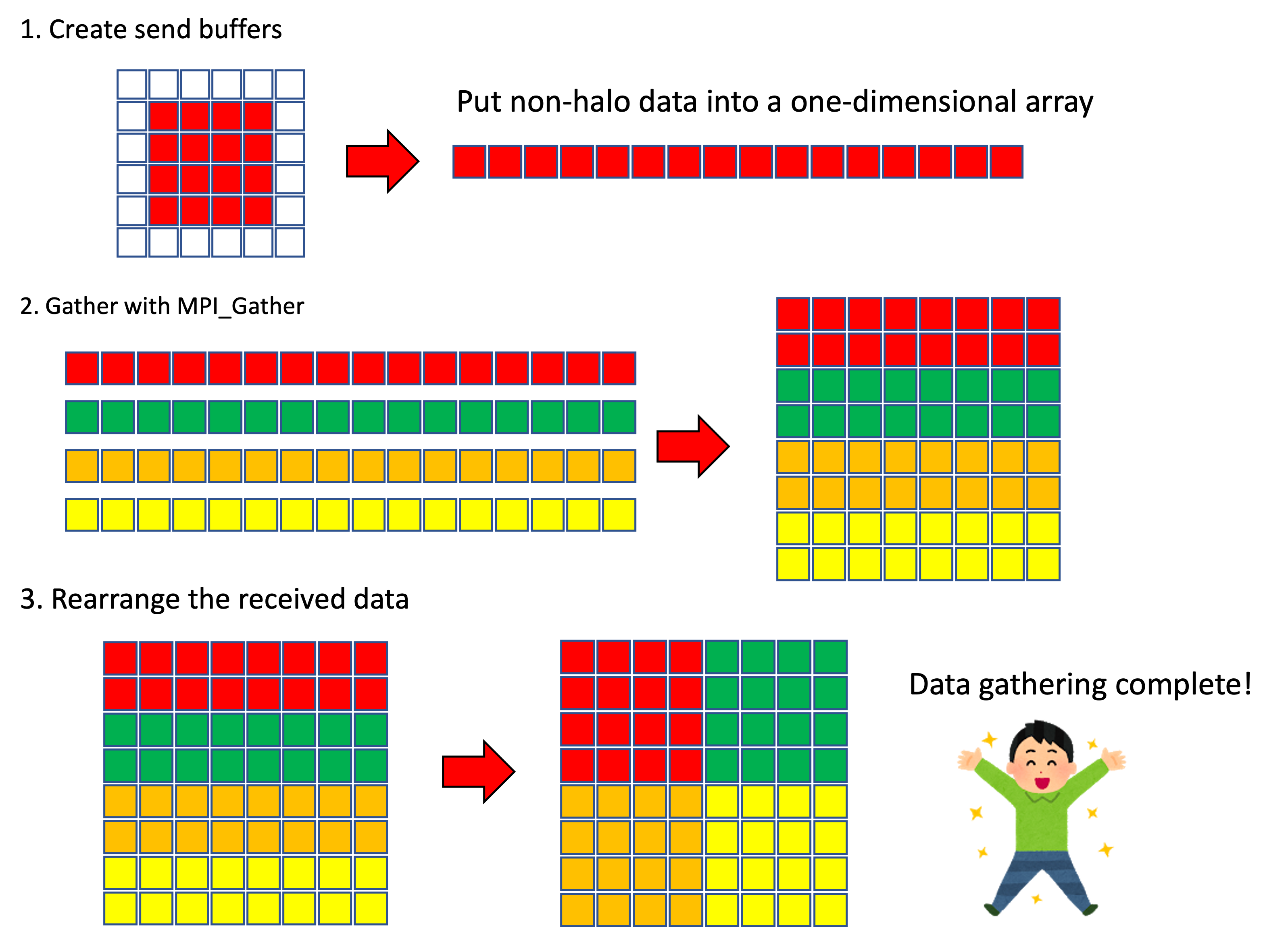
To save the time-evolved result, gather the data held by all processes. We will call the data on each process local data and the complete system data global data. Halos are needed for calculation but not for saving. Each process therefore first extracts its local data without halos, then uses MPI_Gather to collect it on the root process.

Suppose the processes hold data as follows.

rank = 0
 000 000 000 000 000 000
 000 000 001 002 003 000
 000 004 005 006 007 000
 000 008 009 010 011 000
 000 012 013 014 015 000
 000 000 000 000 000 000

rank = 1
 000 000 000 000 000 000
 000 016 017 018 019 000
 000 020 021 022 023 000
 000 024 025 026 027 000
 000 028 029 030 031 000
 000 000 000 000 000 000

rank = 2
 000 000 000 000 000 000
 000 032 033 034 035 000
 000 036 037 038 039 000
 000 040 041 042 043 000
 000 044 045 046 047 000
 000 000 000 000 000 000

rank = 3
 000 000 000 000 000 000
 000 048 049 050 051 000
 000 052 053 054 055 000
 000 056 057 058 059 000
 000 060 061 062 063 000
 000 000 000 000 000 000

The zeros are halo values. Although the global domain is decomposed in two dimensions, each process stores its portion linearly. Apart from copying the data without halos, communication is therefore the same as in one dimension.

void gather(std::vector<int> &local_data, MPIinfo &mi) {
  const int lx = mi.local_size_x;
  const int ly = mi.local_size_y;
  std::vector<int> sendbuf(lx * ly);
  // Copy data excluding halos
  for (int iy = 0; iy < ly; iy++) {
    for (int ix = 0; ix < lx; ix++) {
      int index_from = (ix + 1) + (iy + 1) * (lx + 2);
      int index_to = ix + iy * lx;
      sendbuf[index_to] = local_data[index_from];
    }
  }
  std::vector<int> recvbuf;
  if (mi.rank == 0) {
    recvbuf.resize(lx * ly * mi.procs);
  }
  MPI_Gather(sendbuf.data(), lx * ly, MPI_INT, recvbuf.data(), lx * ly, MPI_INT, 0,  MPI_COMM_WORLD);
  // At this point, recvbuf on rank 0 contains the global data.
}

However, the global data gathered this way are arranged differently from their logical positions on the processes, as shown below.

Before reordering
 000 001 002 003 004 005 006 007
 008 009 010 011 012 013 014 015
 016 017 018 019 020 021 022 023
 024 025 026 027 028 029 030 031
 032 033 034 035 036 037 038 039
 040 041 042 043 044 045 046 047
 048 049 050 051 052 053 054 055
 056 057 058 059 060 061 062 063

The numbers are consecutive because we deliberately initialized the local data that way to simplify debugging. Logically, we want the following arrangement.

After reordering
 000 001 002 003 016 017 018 019
 004 005 006 007 020 021 022 023
 008 009 010 011 024 025 026 027
 012 013 014 015 028 029 030 031
 032 033 034 035 048 049 050 051
 036 037 038 039 052 053 054 055
 040 041 042 043 056 057 058 059
 044 045 046 047 060 061 062 063

We only need to rearrange the data accordingly. A function reordering can perform that operation as follows.

void reordering(std::vector<int> &v, MPIinfo &mi) {
  std::vector<int> v2(v.size());
  std::copy(v.begin(), v.end(), v2.begin());
  const int lx = mi.local_size_x;
  const int ly = mi.local_size_y;
  int i = 0;
  for (int r = 0; r < mi.procs; r++) {
    int rx = r % mi.GX;
    int ry = r / mi.GX;
    int sx = rx * lx;
    int sy = ry * ly;
    for (int iy = 0; iy < ly; iy++) {
      for (int ix = 0; ix < lx; ix++) {
        int index = (sx + ix) + (sy + iy) * L;
        v[index] = v2[i];
        i++;
      }
    }
  }
}

Including these steps, the completed gather function is as follows.

void gather(std::vector<int> &local_data, MPIinfo &mi) {
  const int lx = mi.local_size_x;
  const int ly = mi.local_size_y;
  std::vector<int> sendbuf(lx * ly);
  // Copy data excluding halos
  for (int iy = 0; iy < ly; iy++) {
    for (int ix = 0; ix < lx; ix++) {
      int index_from = (ix + 1) + (iy + 1) * (lx + 2);
      int index_to = ix + iy * lx;
      sendbuf[index_to] = local_data[index_from];
    }
  }
  std::vector<int> recvbuf;
  if (mi.rank == 0) {
    recvbuf.resize(lx * ly * mi.procs);
  }
  MPI_Gather(sendbuf.data(), lx * ly, MPI_INT, recvbuf.data(), lx * ly, MPI_INT, 0,  MPI_COMM_WORLD);
  if (mi.rank == 0) {
    printf("Before reordering\n");
    dump_global(recvbuf);
    reordering(recvbuf, mi);
    printf("After reordering\n");
    dump_global(recvbuf);
  }
}

Because data must be processed before and after transmission, the code is fairly long despite doing something simple. This may explain why MPI is considered cumbersome, and the author will not deny that it is. If you have read this far, however, you will probably agree that MPI is not difficult. MPI does exactly what you write; once the communication algorithm is decided, you implement its steps. The tedious part is often the preprocessing and postprocessing rather than communication itself—in this example, the communication is a single line.

Let gather2d.cpp contain all of the above. Since it is somewhat long, here is a link to the complete source.

https://github.com/kaityo256/sevendayshpc/blob/main/examples/day5/gather2d.cpp

Its main function is shown below.

int main(int argc, char **argv) {
  MPI_Init(&argc, &argv);
  MPIinfo mi;
  setup_info(mi);
  // Allocate local data
  std::vector<int> local_data((mi.local_size_x + 2) * (mi.local_size_y + 2), 0);
  // Initialize local data
  init(local_data, mi);
  // Print local data
  dump_local(local_data, mi);
  // Gather local data into global data
  gather(local_data, mi);
  MPI_Finalize();
}

It simply spells out the procedure directly.

Parallelization Step 2: Halo Exchange

To perform the calculation, each process must receive values for its halos from the processes above, below, left, and right. In two dimensions it also needs corner values—that is, diagonal communication. A straightforward implementation would require eight exchanges: two horizontal, two vertical, and four diagonal. By forwarding horizontally received data in the vertical exchanges, however, diagonal communication can also be completed in only four exchanges.

As an aside, the author once wrote on a now-inactive blog, “How should I handle diagonal communication?” Two readers independently suggested this algorithm (thank you both). Sometimes writing a blog pays off.

The data transfer is illustrated below. First comes horizontal communication. In the actual 2x2 decomposition, the processes to the left and right are the same process, but the figure depicts them separately for clarity.

Communication along the x axis

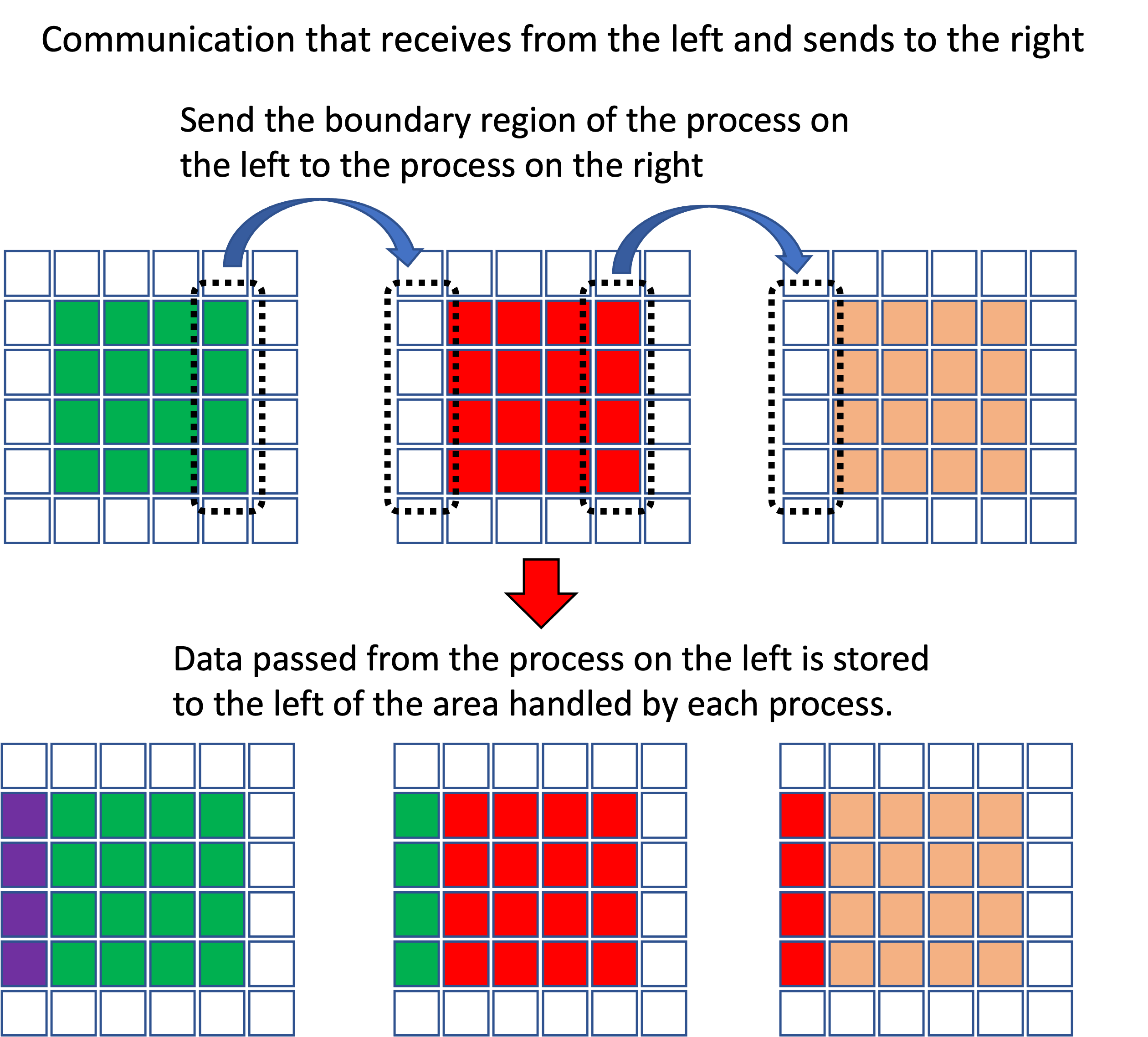
After horizontal communication, transfer data vertically, including the values just received from the left and right. The following exchange receives from below and sends upward.

Communication along the y axis

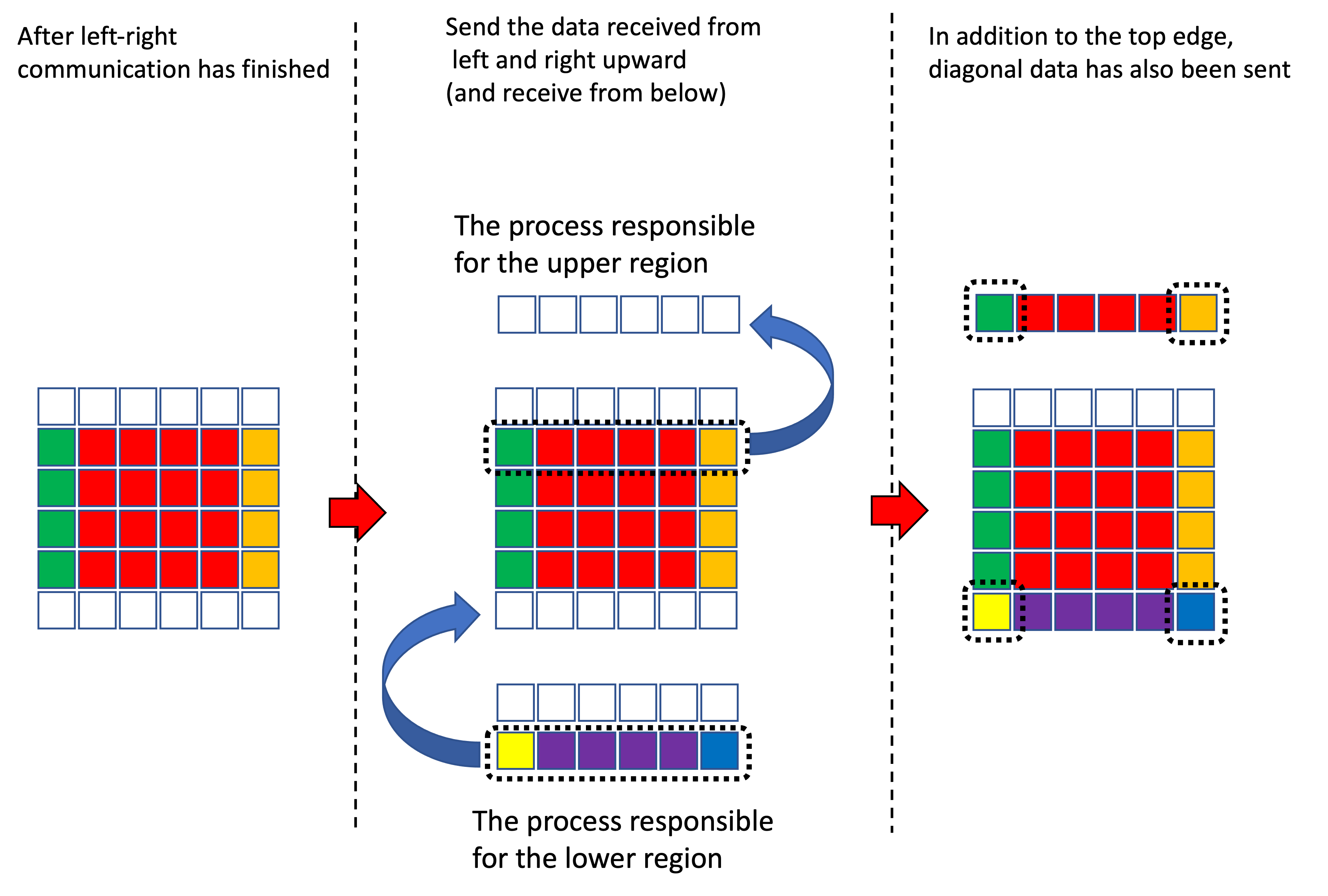
The values enclosed by the final dashed outline originated on a diagonally adjacent process and were received indirectly.

First, we need the ranks of the processes above, below, left, and right. Add a get_rank method to MPIinfo.

struct MPIinfo {
  int rank;
  int procs;
  int GX, GY;
  int local_grid_x, local_grid_y;
  int local_size_x, local_size_y;
  // Return the rank offset by (dx,dy) from this process
  int get_rank(int dx, int dy) {
    int rx = (local_grid_x + dx + GX) % GX;
    int ry = (local_grid_y + dy + GY) % GY;
    return rx + ry * GX;
  }
};

Using this method, the code that communicates horizontally and exchanges left and right halo values is as follows.

void sendrecv_x(std::vector<int> &local_data, MPIinfo &mi) {
  const int lx = mi.local_size_x;
  const int ly = mi.local_size_y;
  std::vector<int> sendbuf(ly);
  std::vector<int> recvbuf(ly);
  int left = mi.get_rank(-1, 0);
  int right = mi.get_rank(1, 0);
  for (int i = 0; i < ly; i++) {
    int index = lx + (i + 1) * (lx + 2);
    sendbuf[i] = local_data[index];
  }
  MPI_Status st;
  MPI_Sendrecv(sendbuf.data(), ly, MPI_INT, right, 0,
               recvbuf.data(), ly, MPI_INT, left, 0, MPI_COMM_WORLD, &st);
  for (int i = 0; i < ly; i++) {
    int index = (i + 1) * (lx + 2);
    local_data[index] = recvbuf[i];
  }

  for (int i = 0; i < ly; i++) {
    int index = 1 + (i + 1) * (lx + 2);
    sendbuf[i] = local_data[index];
  }
  MPI_Sendrecv(sendbuf.data(), ly, MPI_INT, left, 0,
               recvbuf.data(), ly, MPI_INT, right, 0, MPI_COMM_WORLD, &st);
  for (int i = 0; i < ly; i++) {
    int index = lx + 1 + (i + 1) * (lx + 2);
    local_data[index] = recvbuf[i];
  }
}

Vertical communication is nearly identical, except that it also forwards the data received horizontally, as explained above.

An implementation of this algorithm is available here.

https://github.com/kaityo256/sevendayshpc/blob/main/examples/day5/sendrecv.cpp

The output is as follows.

$ mpic++ sendrecv.cpp
$ mpirun -np 4 ./a.out

# Before communication
rank = 0
 000 000 000 000 000 000
 000 000 001 002 003 000
 000 004 005 006 007 000
 000 008 009 010 011 000
 000 012 013 014 015 000
 000 000 000 000 000 000

rank = 1
 000 000 000 000 000 000
 000 016 017 018 019 000
 000 020 021 022 023 000
 000 024 025 026 027 000
 000 028 029 030 031 000
 000 000 000 000 000 000

rank = 2
 000 000 000 000 000 000
 000 032 033 034 035 000
 000 036 037 038 039 000
 000 040 041 042 043 000
 000 044 045 046 047 000
 000 000 000 000 000 000

rank = 3
 000 000 000 000 000 000
 000 048 049 050 051 000
 000 052 053 054 055 000
 000 056 057 058 059 000
 000 060 061 062 063 000
 000 000 000 000 000 000

# After horizontal communication

rank = 0
 000 000 000 000 000 000
 019 000 001 002 003 016
 023 004 005 006 007 020
 027 008 009 010 011 024
 031 012 013 014 015 028
 000 000 000 000 000 000

rank = 1
 000 000 000 000 000 000
 003 016 017 018 019 000
 007 020 021 022 023 004
 011 024 025 026 027 008
 015 028 029 030 031 012
 000 000 000 000 000 000

rank = 2
 000 000 000 000 000 000
 051 032 033 034 035 048
 055 036 037 038 039 052
 059 040 041 042 043 056
 063 044 045 046 047 060
 000 000 000 000 000 000

rank = 3
 000 000 000 000 000 000
 035 048 049 050 051 032
 039 052 053 054 055 036
 043 056 057 058 059 040
 047 060 061 062 063 044
 000 000 000 000 000 000

# After vertical communication (diagonal exchange is now also complete)

rank = 0
 063 044 045 046 047 060
 019 000 001 002 003 016
 023 004 005 006 007 020
 027 008 009 010 011 024
 031 012 013 014 015 028
 051 032 033 034 035 048

rank = 1
 047 060 061 062 063 044
 003 016 017 018 019 000
 007 020 021 022 023 004
 011 024 025 026 027 008
 015 028 029 030 031 012
 035 048 049 050 051 032

rank = 2
 031 012 013 014 015 028
 051 032 033 034 035 048
 055 036 037 038 039 052
 059 040 041 042 043 056
 063 044 045 046 047 060
 019 000 001 002 003 016

rank = 3
 015 028 029 030 031 012
 035 048 049 050 051 032
 039 052 053 054 055 036
 043 056 057 058 059 040
 047 060 061 062 063 044
 003 016 017 018 019 000

Compare it with the preceding figures and verify that communication occurred correctly.

Ultimately, a communication program performs these steps:

Prepare send and receive buffers.
Copy outgoing data into the send buffer.
Communicate.
Copy data from the receive buffer to where it is needed.

Communication itself is a single function call and is neither hard nor tedious; managing the send and receive buffers is the tedious part.

Parallelization Step 3: Implementing the Parallel Code

Now that we have verified the communication algorithm, we can implement it in the finite-difference code. First consider initialization. We want to describe initialization in global coordinates, but the values must be stored in each process’s local data. We therefore need to ask, “Is this global coordinate inside my region?” and, if so, “What is its local index?” Add methods for these operations to MPIinfo.

struct MPIinfo {
  int rank;
  int procs;
  int GX, GY;
  int local_grid_x, local_grid_y;
  int local_size_x, local_size_y;

  // Return the rank offset by +dx, +dy from this process
  int get_rank(int dx, int dy) {
    int rx = (local_grid_x + dx + GX) % GX;
    int ry = (local_grid_y + dy + GY) % GY;
    return rx + ry * GX;
  }

  // Whether a point belongs to this process's region
  bool is_inside(int x, int y) {
    int sx = local_size_x * local_grid_x;
    int sy = local_size_y * local_grid_y;
    int ex = sx + local_size_x;
    int ey = sy + local_size_y;
    if (x < sx)return false;
    if (x >= ex)return false;
    if (y < sy)return false;
    if (y >= ey)return false;
    return true;
  }
  // Convert global coordinates to a local index
  int g2i(int gx, int gy) {
    int sx = local_size_x * local_grid_x;
    int sy = local_size_y * local_grid_y;
    int x = gx - sx;
    int y = gy - sy;
    return (x + 1) + (y + 1) * (local_size_x + 2);
  }
};

Initialization can then be written as follows.

void init(vd &u, vd &v, MPIinfo &mi) {
  int d = 3;
  for (int i = L / 2 - d; i < L / 2 + d; i++) {
    for (int j = L / 2 - d; j < L / 2 + d; j++) {
      if (!mi.is_inside(i, j)) continue;
      int k = mi.g2i(i, j);
      u[k] = 0.7;
    }
  }
  d = 6;
  for (int i = L / 2 - d; i < L / 2 + d; i++) {
    for (int j = L / 2 - d; j < L / 2 + d; j++) {
      if (!mi.is_inside(i, j)) continue;
      int k = mi.g2i(i, j);
      v[k] = 0.9;
    }
  }
}

The code loops over global coordinates; whenever a point belongs to this process (mi.is_inside(i, j)==true), it obtains the local index and stores the value there. Looping over points outside the owned region may seem inefficient, but initialization runs only once. This design is convenient because other initial conditions, or initialization from a file, can use the same input for serial and parallel programs.

After initialization, write the file-output code used for visualization. This merely changes the code from Step 2 from int to double and saves to a file instead of standard output.

// Receive data from all processes and save it
void save_as_dat_mpi(vd &local_data, MPIinfo &mi) {
  const int lx = mi.local_size_x;
  const int ly = mi.local_size_y;
  vd sendbuf(lx * ly);
  // Copy data excluding halos
  for (int iy = 0; iy < ly; iy++) {
    for (int ix = 0; ix < lx; ix++) {
      int index_from = (ix + 1) + (iy + 1) * (lx + 2);
      int index_to = ix + iy * lx;
      sendbuf[index_to] = local_data[index_from];
    }
  }
  vd recvbuf;
  if (mi.rank == 0) {
    recvbuf.resize(lx * ly * mi.procs);
  }
  MPI_Gather(sendbuf.data(), lx * ly, MPI_DOUBLE, recvbuf.data(), lx * ly, MPI_DOUBLE, 0,  MPI_COMM_WORLD);
  if (mi.rank == 0) {
    reordering(recvbuf, mi);
    save_as_dat(recvbuf);
  }
}

Data rearrangement (reordering) is almost identical and is omitted. At this point, do not begin time evolution immediately. Initialize the system, save it, and verify that initialization and output are correct.

The halo-exchange code also differs mainly by changing int to double, so it is omitted. Both u and v must be exchanged, however, so define a function that handles them together.

void sendrecv(vd &u, vd &v, MPIinfo &mi) {
  sendrecv_x(u, mi);
  sendrecv_y(u, mi);
  sendrecv_x(v, mi);
  sendrecv_y(v, mi);
}

Calling this immediately before time evolution completes the halo exchange. Again, do not begin time evolution immediately. Initialize the data, perform halo exchange, dump the local arrays, and verify that communication is correct.

Once these checks pass, the remainder is nearly identical to the serial version. The main function is as follows.

int main(int argc, char **argv) {
  MPI_Init(&argc, &argv);
  MPIinfo mi;
  setup_info(mi);
  const int V = (mi.local_size_x + 2) * (mi.local_size_y + 2);
  vd u(V, 0.0), v(V, 0.0);
  vd u2(V, 0.0), v2(V, 0.0);
  init(u, v, mi);
  for (int i = 0; i < TOTAL_STEP; i++) {
    if (i & 1) {
      sendrecv(u2, v2, mi);
      calc(u2, v2, u, v, mi);
    } else {
      sendrecv(u, v, mi);
      calc(u, v, u2, v2, mi);
    }
    if (i % INTERVAL == 0) save_as_dat_mpi(u, mi);
  }
  MPI_Finalize();
}

Apart from MPI initialization and finalization and the communication call before each update, it is unchanged from the serial version.

Let us run it. On the author’s system, ordinary mpic++ invokes clang++. To compare execution time with the serial version compiled earlier using g++, explicitly compile this program with g++ as well. The MPI headers and libraries are on the author’s search paths, so adding -lmpi -lmpi_cxx is sufficient.

$ g++ -O3 gs_mpi.cpp -lmpi -lmpi_cxx
$ time mpirun -np 4 --oversubscribe ./a.out
conf000.dat
conf001.dat
conf002.dat
(snip)
conf098.dat
conf099.dat
mpirun -np 4 --oversubscribe ./a.out  2.39s user 0.29s system 321% cpu 0.832 total

The percentage reported by time indicates CPU-core utilization; fully using one core is 100%. Here it reports 321%, confirming a parallel calculation using roughly four cores. Execution also became nearly twice as fast, from 1.697 s to 0.832 s.

Suppose the serial and MPI versions were run in directories named serial and mpi, each containing its data files. Compare them with diff. Before time evolution, the results are naturally identical.

$ diff -s serial/conf000.dat mpi/conf000.dat
Files serial/conf000.dat and mpi/conf000.dat are identical

From the next step onward, however, they diverge because of floating-point error.

$ diff -s serial/conf001.dat mpi/conf001.dat
Binary files serial/conf001.dat and mpi/conf001.dat differ

This occurs because the order of additions differs between the serial and MPI versions. The calculations are essentially equivalent, so visualization should produce similar patterns. Let us check.

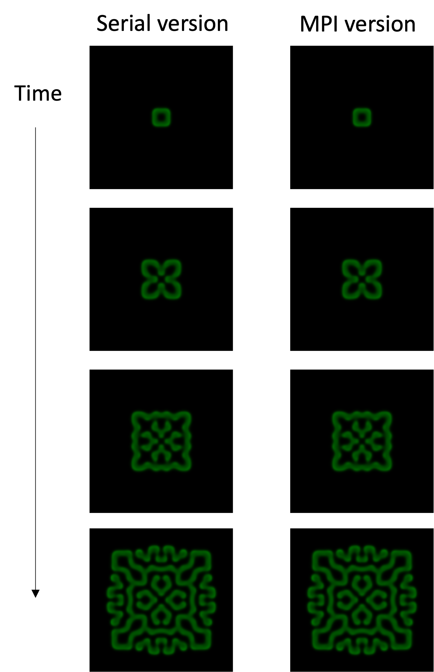
Comparison of time evolution in the serial and MPI versions

Yes, the results look fine.

Execution time improved from 1.697 s to 0.832 s, nearly a factor of two, but we used four CPU cores. Ideally it would be four times faster; a speedup of only about two means a parallel efficiency of roughly 50%.

What, the parallel efficiency seems disappointing? Then retreat to weak scaling and overwhelm the problem with size.

Increase each side by a factor of four and run it again.

const int L = 128;
const int L = 512;

$ g++ -O3 gs.cpp
$ time ./a.out
(snip)
./a.out  57.98s user 0.16s system 99% cpu 58.248 total

$ g++ -O3 gs_mpi.cpp -lmpi -lmpi_cxx
$ time mpirun -np 4 --oversubscribe ./a.out
./a.out  57.98s user 0.16s system 99% cpu 58.248 total
mpirun -np 4 --oversubscribe ./a.out  68.28s user 1.72s system 382% cpu 18.305 total

Execution time falls from 58.248 s to 18.305 s, raising parallel efficiency to nearly 80%. If anyone still complains, calculate a system far too large to fit in a local PC’s memory. Remember: when parallel efficiency troubles you, escape by increasing the problem size.

Aside: The Tediousness of MPI

As a realistic domain-decomposition example, we parallelized a two-dimensional reaction-diffusion equation. Let us see how much code parallelization added.

$ wc gs.cpp gs_mpi.cpp
      89     430    1969 gs.cpp
     272    1271    7345 gs_mpi.cpp
     361    1701    9314 total

The program grew from 89 lines to 272—roughly threefold. In other words, communication-related code twice the size of the original calculation was added. Yet the actual communication calls occupy very little code.

$ grep MPI_ gs_mpi.cpp
  MPI_Comm_rank(MPI_COMM_WORLD, &rank);
  MPI_Comm_size(MPI_COMM_WORLD, &procs);
  MPI_Dims_create(procs, 2, d2);
  MPI_Gather(sendbuf.data(), lx * ly, MPI_DOUBLE, recvbuf.data(), lx * ly, MPI_DOUBLE, 0,  MPI_COMM_WORLD);
  MPI_Status st;
  MPI_Sendrecv(sendbuf.data(), ly, MPI_DOUBLE, right, 0,
               recvbuf.data(), ly, MPI_DOUBLE, left, 0, MPI_COMM_WORLD, &st);
  MPI_Sendrecv(sendbuf.data(), ly, MPI_DOUBLE, left, 0,
               recvbuf.data(), ly, MPI_DOUBLE, right, 0, MPI_COMM_WORLD, &st);
  MPI_Status st;
  MPI_Sendrecv(sendbuf.data(), lx + 2, MPI_DOUBLE, up, 0,
               recvbuf.data(), lx + 2, MPI_DOUBLE, down, 0, MPI_COMM_WORLD, &st);
  MPI_Sendrecv(sendbuf.data(), lx + 2, MPI_DOUBLE, down, 0,
               recvbuf.data(), lx + 2, MPI_DOUBLE, up, 0, MPI_COMM_WORLD, &st);
  MPI_Init(&argc, &argv);
  MPI_Finalize();

$ grep MPI_ gs_mpi.cpp | wc
      16      82     850

Excluding the declaration of MPI_Status st, there are only 14 lines. Everything else prepares and organizes buffers. If this is what one means by “MPI is tedious,” the author agrees. But this is not the true source of MPI’s difficulty.

Writing parallel code with MPI is called parallelization. The word may suggest modifying an existing serial program into a parallel one. A typical development process tends to be:

Write serial code.
When a larger system is needed, add thread parallelism with OpenMP.
Modify it further into an MPI-parallel version.

Retrofitting MPI into existing code, however, is extremely tedious, prone to bugs, and likely to leave you unsure what the program is doing. Once that happens, it becomes impossible to tell where a bug is or what caused it, and the project sinks into a quagmire. The author has repeatedly seen this happen not only to students but also to professional programmers.

Thread parallelism aside, parallelizing with MPI means rewriting the program as new MPI-oriented code. A sound process is:

Write serial code.
Identify the communication patterns required for MPI parallelization.
Write a test program containing only those communication patterns.
Develop a new program while referring to both the serial and test code.

In step 4 specifically, we initialized, gathered, and saved the data and verified correctness; then initialized, exchanged halos, and verified correctness before proceeding. The parallel gs_mpi.cpp was developed from scratch with reference to the serial gs.cpp, not by copying it. MPI is tedious—that feeling is correct—but it is not difficult when development proceeds systematically. Tripling the source size may sound alarming, yet the result is still under 300 lines, and writing the communication calls does not take long. As in all programming, most development time is spent debugging. If you take the trouble to write proper tests for the communication logic, parallelization should not take very long.

What if someone hands you 20,000 lines of source code and says, “Parallelize this”? In that case, all we can offer is our condolences…